RHIP

Receding Horizon Inverse Planning is a horizon-parameterised inverse reinforcement learning estimator. It recovers a linear reward by matching discounted feature expectations, with a single hyperparameter, the planning horizon \(H\), controlling how far the agent plans with the stochastic soft-Bellman policy before falling back to a deterministic planner. The horizon spans a family of classic methods: at \(H = \infty\) it is maximum causal entropy IRL, at \(H = 0\) it is the Max-Margin-Planning end, and intermediate values interpolate.

Read this page when the demonstrator may not be an infinite-horizon planner. The horizon changes the behavioral model being matched; it is not a new source of reward identification by itself.

Source Papers

The estimator follows Barnes et al. (2024), which introduces receding horizon inverse planning and shows that the planning horizon spans maximum causal entropy IRL, a Bayesian-IRL-like middle ground, and Max-Margin Planning as special cases. The infinite-horizon endpoint coincides with maximum causal entropy IRL, following Ziebart (2010). The package replicates the method, the horizon spectrum, not the planetary-scale graph machinery of the source application.

Notation

Throughout, \(s\) indexes the discrete state and \(a\) the discrete action, observed for individual \(i\) in period \(t\). The vector \(\phi(s, a)\) collects the action-dependent reward features and \(\theta\) the reward parameters to be estimated. The discount factor is \(\beta\) and the logit shock scale is \(\sigma\). The transition kernel \(P_a(s, s')\) gives the probability of moving to \(s'\) from \(s\) under action \(a\), stored in \((A, S, S)\) orientation. The planning horizon is \(H\). The deterministic continuation value is \(V^{\mathrm{det}}(s)\), the horizon-\(H\) soft value is \(V_H(s)\), the choice-specific value is \(Q_H(s, a)\), and the receding-horizon policy is \(\pi_H(a \mid s)\). The empirical discounted feature occupancy is \(\mu_E\) and the model occupancy under \(\pi_H\) is \(\mu_H\).

Model

The observed data are state, action, and next-state trajectories \((s_{it}, a_{it}, s_{i,t+1})\). The reward is linear in the action-dependent features:

\[ r_\theta(s, a) = \phi(s, a)^\top \theta. \]

Beyond the planning horizon the agent uses a cheap deterministic planner. The continuation value is the hard-max optimum, the \(\sigma \to 0\) limit of the soft operator:

\[ V^{\mathrm{det}}(s) = \max_a \left[ r_\theta(s, a) + \beta \sum_{s'} P_a(s, s')\, V^{\mathrm{det}}(s') \right]. \]

Within the horizon, \(H\) soft-Bellman backups run on top of \(V^{\mathrm{det}}\). Starting from \(V_0 = V^{\mathrm{det}}\), for \(k = 1, \dots, H\):

\[ Q_k(s, a) = r_\theta(s, a) + \beta \sum_{s'} P_a(s, s')\, V_{k-1}(s'), \qquad V_k(s) = \sigma \log \sum_a \exp\!\left(\frac{Q_k(s, a)}{\sigma}\right). \]

The receding-horizon policy is the softmax of the final choice-specific values:

\[ \pi_H(a \mid s) = \frac{\exp(Q_H(s, a) / \sigma)}{\sum_b \exp(Q_H(s, b) / \sigma)}. \]

At \(H = 0\) no soft backups run, so the policy is the softmax over the deterministic continuation value, the Max-Margin-Planning end. As \(H \to \infty\) the soft backups drive \(V\) to the soft fixed point, the maximum causal entropy end. The canonical instance is route choice on a road network: a traveller moves one edge at a time, and the planning horizon sets how far ahead the route is planned stochastically.

Identification

This is the section that says what must hold before the horizon-specific moment match can be read as reward recovery.

RHIP recovers a reward representation under the maximum causal entropy dynamic discrete choice assumptions. These are inherited unchanged from MCE-IRL; the horizon \(H\) is a planner hyperparameter, not an identifying assumption.

Known transitions. The transition kernel \(P_a(s, s')\) is supplied or estimated outside the estimator and does not depend on the reward parameters.
Causal behavioral model. The agent’s policy is the soft-optimal causal policy. The action distribution at each state is the softmax of the choice-specific values from the soft Bellman recursion.
Additive linear reward. The reward is linear in the supplied feature matrix: \(r_\theta(s, a) = \phi(s, a)^\top \theta\). Structural counterfactuals require this parametric form.
Reward normalization. The reward is identified only up to transformations that leave behavior unchanged, including additive constants and reward shaping. A normalization anchor must be applied consistently when comparing estimated and reference rewards.
Action-dependent feature rank. The feature design must vary across actions. State-only features broadcast across actions and leave action-specific payoff differences unidentified.
Sufficient action support. Each action must have enough observed support for the occupancy comparison. Thin support leaves the corresponding reward directions weakly pinned.

These hold inside a finite discrete state space with a stationary environment and a known discount factor \(\beta\). Under them, the feature-moment condition \(\mu_E = \mu_H\) determines \(\theta\) within the supplied feature basis and normalization. The horizon \(H\) selects which behavioral model the moments are matched against, namely how far the agent plans stochastically, so a horizon that fits the demonstrator-noise regime improves recovery. It adds no identification restriction. At \(H = \infty\) the assumption set is exactly that of maximum causal entropy IRL.

Estimator

RHIP matches discounted feature expectations. The empirical and model feature moments are:

\[ \mu_E = \sum_{s,a} D_E(s, a)\,\phi(s, a), \qquad \mu_H = \sum_{s,a} D_H(s, a)\,\phi(s, a), \]

where \(D_E\) is the empirical discounted occupancy and \(D_H\) is the occupancy induced by \(\pi_H\). The estimator ascends the maximum-entropy feature-matching gradient:

\[ \nabla_\theta L(\theta) = \mu_E - \mu_H. \]

This is the same gradient form as MCE-IRL. The horizon changes only the policy \(\pi_H\) that drives the model occupancy \(D_H\), not the gradient. The empirical occupancy, the initial distribution, and the forward state-visitation fixed point are computed by the shared MCE-IRL occupancy helpers.

Algorithm

Algorithm  RHIP (receding-horizon feature matching, finite H)
Input   panel {(s_it, a_it, s_{i,t+1})}, features phi, transitions P,
        discount beta, logit scale sigma, horizon H
Output  theta_hat, policy pi_H, value V_H

 compute empirical feature moments mu_E from the demonstration occupancy
 compute initial state distribution rho_0 from the data
 initialize theta
 repeat                                         # outer loop: Adam ascent
     r_theta(s, a) := phi(s, a)' theta
     V_det := hard-max value iteration under r_theta      # deterministic tail
     V_0 := V_det
     for k = 1..H:                              # H soft-Bellman backups
         Q_k(s, a) := r_theta(s, a) + beta * sum_{s'} P_a(s, s') V_{k-1}(s')
        V_k(s)    := sigma * logsumexp_a Q_k(s, a) / sigma
    pi_H(a | s)   := exp(Q_H(s, a)/sigma) / sum_b exp(Q_H(s, b)/sigma)
    D_H           := forward state-visitation fixed point under pi_H, rho_0
    mu_H          := sum_{s,a} D_H(s, a) phi(s, a)
    grad          := mu_E - mu_H
    update theta by Adam along grad
until the gradient norm or the occupancy moment is below tolerance
return theta_hat, pi_H, V_H

The infinite-horizon endpoint takes a separate path. When horizon=float("inf") (or None), RHIP uses the MCE-IRL endpoint, so \(H = \infty\) reproduces maximum causal entropy IRL exactly with the same config. At finite \(H\) the deterministic tail in step 6 is plain hard-max value iteration, and \(H = 0\) runs no soft backups so the policy is the softmax over the deterministic continuation value. The implementation lives in econirl.estimators.rhip.

Applicability

Applicable when	Prefer an alternative when
Demonstrations come from a discrete sequential decision problem.	Likelihood-based structural standard errors are required.
Transitions are known or can be supplied.	Transition estimation is the main modeling challenge.
Reward features are supplied and action-dependent.	Reward features are unknown or require a neural representation.
The full stochastic planner is too costly at scale.	A small state space makes the full soft solve cheap.
A tunable planning horizon between deterministic and stochastic is wanted.	A single fixed behavioral model is sufficient.

RHIP sits across the entropy IRL family. At \(H = \infty\) it coincides with MCE-IRL, the reference entropy IRL estimator. At \(H = 0\) it occupies the Max-Margin-Planning end of the spectrum, fully deterministic and cheap. Intermediate horizons interpolate between the two. The structural estimators (NFXP, CCP, MPEC) target the same reward through likelihood paths and report standard errors for \(\theta\), which RHIP does not.

Usage

RHIP fits a pre-built panel with action-dependent features and a transition tensor in \((A, S, S)\) orientation:

import numpy as np

from econirl import RHIP

model = RHIP(horizon=3, discount=0.95, scale=1.0,
            feature_names=["edge_cost", "amenity", "goal"])
model.fit(panel, features=features, transitions=transitions)

print(model.params_)
print(model.policy_.shape)

The horizon is the single knob. horizon=float("inf") recovers maximum causal entropy IRL; horizon=0 is the deterministic end:

mce = RHIP(horizon=float("inf"))      # the MCE-IRL endpoint
mce.fit(panel, features=features, transitions=transitions)

mmp_end = RHIP(horizon=0)             # the Max-Margin-Planning end
mmp_end.fit(panel, features=features, transitions=transitions)

Counterfactual analysis re-solves the dynamic program under changed primitives. The fitted primitives for this are model.reward_matrix_, model.policy_, and model.value_. The fitted policy gives action probabilities by state:

print(model.predict_proba([0, 10, 50, 89]))

Evidence

RHIP is an inverse reinforcement learning estimator, so the reward is identified only up to behavior-preserving transformations. Recovery is measured by behavioral metrics, not parameter bias. The evidence is the single-regime horizon spectrum from the high-dimensional route-choice study: a 150-node random geometric road network with linear reward features \([\text{edge\_cost}, \text{amenity}, \text{goal}]\) and true parameters \(\theta = [1.0, 0.5, 1.0]\). The horizon sweeps \(H \in \{0, 1, 3, \infty\}\).

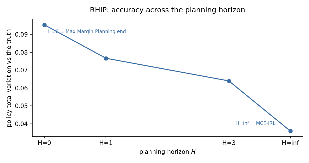
The figure traces policy total variation across the four horizons. Accuracy improves smoothly as the horizon grows, and \(H = \infty\) matches maximum causal entropy IRL.

Policy total variation across the planning horizon

Behavioral recovery and baseline counterfactual regret per horizon, averaged over the study replications:

Horizon	Policy TV	Value RMSE	Baseline regret	Note
\(H = 0\)	0.0952	19.53	0.0519	Max-Margin-Planning end
\(H = 1\)	0.0766	18.34	0.0397	one soft backup
\(H = 3\)	0.0640	15.10	0.0201	middle of the spectrum
\(H = \infty\)	0.0360	3.73	0.0537	matches MCE-IRL

Policy total variation is the distance between the estimated and true choice probabilities, lower is better. It falls monotonically as the horizon grows. At \(H = \infty\) is the MCE-IRL endpoint, so its row matches MCE-IRL by construction. The figure is accuracy-only. Wall-clock fit time is not shown, because the \(H = \infty\) path reuses the optimized MCE-IRL solver and runs faster than the finite-horizon path here, which would invert the planning cost the horizon is meant to trade. For the full cross-estimator comparison, see the high-dimensional route-choice simulation study.

The horizon is an identifiable behavioral parameter, not only a compute knob. A companion study draws demonstrations from a finite-lookahead planner with a true lookahead \(h\), then fits RHIP across a sweep of horizons. The best-fitting horizon recovers the demonstrator’s lookahead: the lowest-error horizon lands at \(H = h\) and tracks \(h\) as it changes, and both the myopic \(H = 0\) and the fully stochastic \(H = \infty\) ends are worse. An interior horizon is the better- specified model when the demonstrator plans neither one step nor infinitely far ahead. See the horizon-recovery simulation study.

References

Source papers:

Barnes, M., Abueg, M., Lange, O. F., Deeds, M., Trader, J., Molitor, D., Wulfmeier, M., and O’Banion, S. (2024). Massively Scalable Inverse Reinforcement Learning in Google Maps. International Conference on Learning Representations. arXiv:2305.11290. reference entry.
Ziebart, B. D. (2010). Modeling Purposeful Adaptive Behavior with the Principle of Maximum Causal Entropy. PhD thesis, Carnegie Mellon University. reference entry.

Implementation and reproduction:

Estimator source and sklearn wrapper: econirl.estimators.rhip.
Infinite-horizon endpoint: econirl.estimation.mce_irl.
Study script: scripts/study_highdim_route_choice.py.
Endpoint-equivalence test: tests/test_rhip.py.
Results file: study_highdim_route_choice.json.

Studies:

Pages: