Consumer stockpiling of a storable good

Read this page as a dynamic inventory benchmark. The important question is whether the recovered model captures forward-looking buying before future high prices, not just current purchase shares.

A household buys a storable good over time. It consumes one unit each period. The shelf price swings between a low sale price and a high regular price. The household can buy a pack now to avoid paying the high price later. The cost of doing so is the holding cost on the inventory it carries.

The data-generating process

The state is a pair: inventory \(i\) and price regime \(p\). Inventory runs from 0 to 9 units. The price regime is sale or regular and follows a two-state Markov chain. Sales are short. Regular spells are longer. The flat state index is \(s = 2i + p\), giving 20 states.

Each period the household chooses to buy a pack of 3 units or not. Then it consumes one unit if any is on hand. Inventory carried to the next period is the post-purchase stock minus one, capped at 9.

The reward is linear in three features:

\[ u_\theta(s, a) = \theta_{\mathrm{spend}}\,(-c_p B a) + \theta_{\mathrm{hold}}\,(-i') + \theta_{\mathrm{stock}}\,(-\mathbf{1}\{i + B a = 0\}) \]

where \(c_p\) is the per-unit price (1 on sale, 2 regular), \(B = 3\) is the pack size, \(a \in \{0, 1\}\) is the buy decision, \(i'\) is the inventory carried forward, and the last term is a stockout penalty paid when the household wanted a unit but had none. The true parameters are \(\theta = [1.0,\;0.2,\;3.0]\).

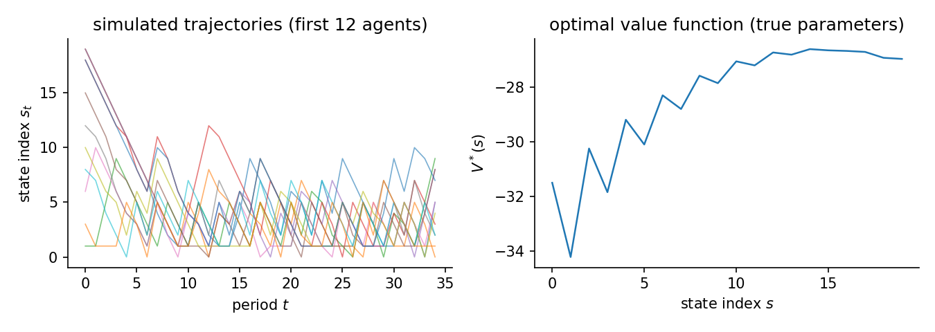
Agents discount future payoffs at \(\beta\) and face i.i.d. logit taste shocks (scale \(\sigma = 1\)). Their behaviour solves the soft Bellman equation. The stockout feature is action-dependent, because buying when inventory is empty avoids the penalty, so all three parameters are identified from observed purchases. The optimal policy stockpiles: it buys more often on sale than at the regular price, at every inventory level, and buys less as inventory rises. The panel simulates \(N\) agents for \(T\) periods from the true optimal policy. The figure shows simulated inventory-price paths and the optimal value function.

The study uses 200 households, 35 periods, and 30 replications. The true parameters are \([1.0,\;0.2,\;3.0]\) for spending, inventory holding, and stockout cost. The action-contrast feature matrix has full rank, so all three parameters are identified from purchases.

Estimators and data

Estimator	Family	Uses transitions \(P(s'\mid s,a)\)	Transferable reward	Standard errors
NFXP	structural	yes	yes	yes
CCP	structural	yes	yes	yes
MCE-IRL	behavioral	yes	yes	no
GLADIUS	behavioral	no	no	no

Uses transitions is whether the estimator reads the transition kernel; model-free learners do not. Transferable reward is whether it recovers a reward that re-solves under a counterfactual. Standard errors is whether it returns inference. The last two are read from the run.

Results

Estimator	Family	Ran	Conv	Recovered params	Param RMSE	Policy TV	Regret base	Regret A	Regret B	Regret C	Time (s)
NFXP	structural	2/2	2/2	[0.993, 0.197, 2.930]	0.0572	0.0026	0.0055	0.0056	0.0010	0.0009	2.4
CCP	structural	2/2	2/2	[0.994, 0.196, 2.930]	0.0572	0.0026	0.0054	0.0055	0.0010	0.0009	2.2
MCE-IRL	behavioral	2/2	0/2	[0.993, 0.197, 2.930]	-	0.0026	0.0055	0.0056	0.0010	0.0009	7.4
GLADIUS	behavioral	2/2	2/2	-	-	0.0647	2.4105	2.5216	5.5947	38.9062	7.5

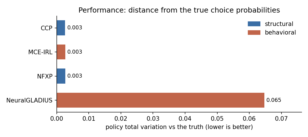
Param RMSE covers the structural family only, which shares the parameterization of the true model. Policy TV is the distance between estimated and true choice probabilities, lower is better. Conv is the estimator’s own convergence indicator. A cautious estimator can report False while the recovered policy is accurate. Regret base is welfare lost in the observed environment. Types A, B, and C are welfare lost after a change. Type A shifts a payoff, Type B changes the transitions, Type C penalizes an action. Estimators with a recovered reward re-solve it and adapt. Those without one keep their old policy.

Parameter recovery

Estimator	Parameter	True	Mean est	Bias	Emp. SE	RMSE	95% coverage	SE avail
NFXP	spend	1.000	0.993	-0.007	0.027	0.020	1.00 +/- 0.00	100% (2 reps)
NFXP	holding	0.200	0.197	-0.003	0.004	0.004	1.00 +/- 0.00	100% (2 reps)
NFXP	stockout	3.000	2.930	-0.070	0.137	0.119	1.00 +/- 0.00	100% (2 reps)
CCP	spend	1.000	0.994	-0.006	0.027	0.020	0.50 +/- 0.35	100% (2 reps)
CCP	holding	0.200	0.196	-0.004	0.004	0.005	1.00 +/- 0.00	100% (2 reps)
CCP	stockout	3.000	2.930	-0.070	0.136	0.119	0.50 +/- 0.35	100% (2 reps)

Coverage is the share of replications whose 95% interval contains the truth, shown with its Monte Carlo standard error. It is computed only where every replication produced a finite standard error. SE avail is the share of replications with finite standard errors.

The structural family (NFXP, CCP, MPEC) recovers all three parameters on the same scale as the truth, so Param RMSE applies to them alone. MCE-IRL here uses the same linear features and recovers the same values, but its weights stay out of the recovery table because an IRL reward is only partially identified in general. GLADIUS learns a neural policy object with no directly comparable reward weights in this study. Policy TV and regret are the right scorecards for the behavioral family.

Reward and structure

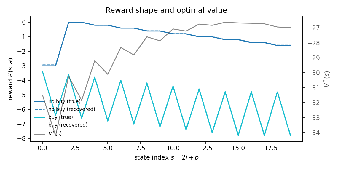
The state index is \(s = 2i + p\): inventory \(i\) rises in steps of two, and the sale and regular price regimes interleave. The reward against \(s\) shows the buy and no-buy lines, with the recovered reward dashed over the true reward. The zigzag is the price regime alternating. The optimal value falls as inventory and holding cost rise.

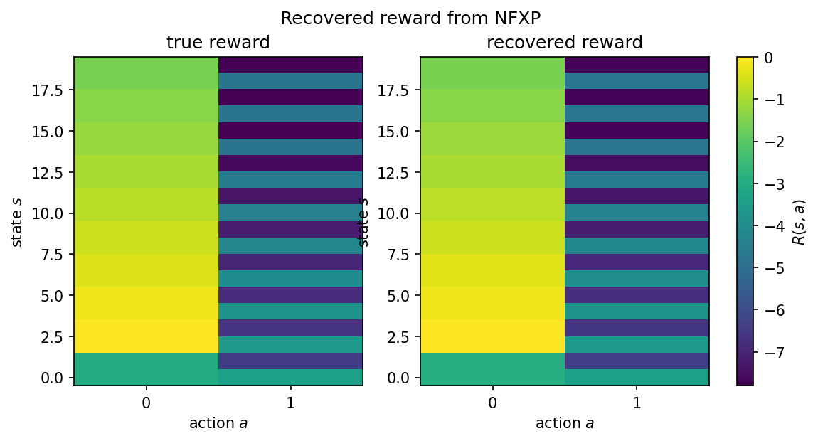
The same reward as a state-by-action heatmap puts the true and recovered rewards side by side on one color scale.

Notes per estimator

NFXP. Full-solution MLE with a nested Bellman fixed-point inner loop. Quadratic convergence near the optimum; all three parameters are identified from the action-dependent stockout feature and the price-varying spending feature.

CCP. CCP uses a first-step nonparametric policy estimate to avoid the inner Bellman loop. One policy-iteration step corrects the bias from the nonparametric first stage.

MCE-IRL. Its convergence indicator mirrors the inner optimizer’s success status. The optimizer can stop short while the recovered policy is already accurate, so it can read False on an accurate fit.

GLADIUS. Neural Q and continuation learner. Uses only the feature matrix and the observed panel; it does not use transition matrices in this study. Capped at 200 epochs here for short compute.

Reproduce

python scripts/study_stockpiling.py                 # run + write JSON
python scripts/study_stockpiling.py --page          # regenerate this page
python scripts/study_stockpiling.py --verify        # re-derive the table from JSON

Results file: validation/results/study_stockpiling.json.

Not shown on this page: MPEC, NNES, SEES, TD-CCP, and UFXP, because NFXP and CCP already cover the structural family on this small stockpiling problem. IQ-Learn and f-IRL are omitted because reward is only partially identified from behavior here. Neural MCE-IRL, neural AIRL, and GLADIUS belong on larger or more reward-flexible studies.