Route choice on a synthetic road network

Read this page as the small graph benchmark. It tests whether estimators recover edge-level reward tradeoffs and counterfactual behavior on a controlled route choice problem.

A traveller moves through a road network one step at a time. Each period, the agent chooses among the nearest neighbours of the current node. The utility depends on the edge: how long it is, how attractive the destination is, and how close the destination sits to a fixed goal node.

The data-generating process

Nodes are scattered uniformly at random in the unit square. Edges connect pairs within a fixed Euclidean radius. A spanning tree is overlaid to keep the graph connected. The agent at node \(s\) picks among \(A\) nearest neighbours sorted by distance. Actions beyond the node degree self-loop.

The reward for traversing edge \((s, a) \to s'\) is linear in three features:

\[ u_\theta(s, a) = \theta_{\mathrm{cost}}\,(-d_{ss'}) + \theta_{\mathrm{am}}\,\mathrm{am}(s') + \theta_{\mathrm{goal}}\,(-\ell_{s'}) \]

where \(d_{ss'}\) is the Euclidean edge length, \(\mathrm{am}(s')\) is a node-level amenity draw, and \(\ell_{s'}\) is the shortest-path distance from \(s'\) to a fixed destination node. The true parameters are \(\theta = [1.0,\;0.5,\;1.0]\).

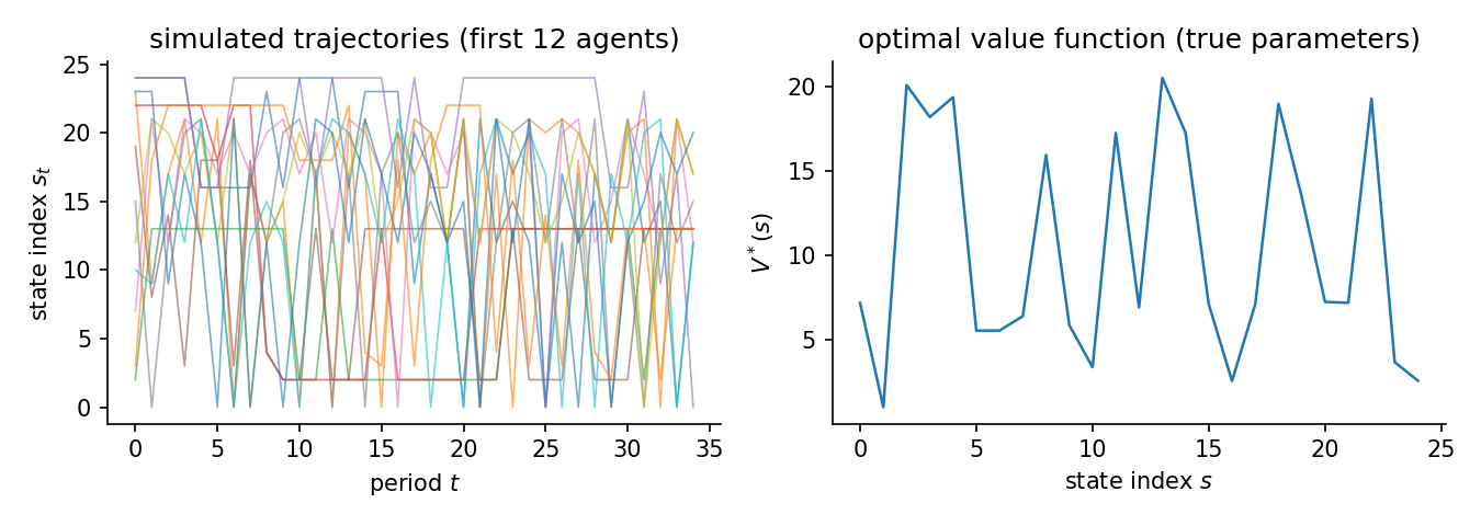
Agents discount future payoffs at \(\beta\) and face i.i.d. logit taste shocks (scale \(\sigma = 1\)). Their behaviour solves the soft Bellman equation. All three parameters are identified from observed route choices because the features vary across edges, not just states. The panel simulates \(N\) agents for \(T\) periods from the true optimal policy. The figure shows simulated paths and the optimal value function (lower at nodes far from the goal).

The study uses a 25-node random geometric road network, 4 actions per node, 200 travellers, 35 periods, and 2 replications. The true reward weights are \([1.0,\;0.5,\;1.0]\). The action-contrast feature matrix has full rank, so the three edge-level reward weights are identifiable from choices.

Estimators and data

Estimator	Family	Uses transitions \(P(s'\mid s,a)\)	Transferable reward	Standard errors
NFXP	structural	yes	yes	yes
CCP	structural	yes	yes	no
MCE-IRL	behavioral	yes	yes	no
GLADIUS	behavioral	no	no	no

Uses transitions is whether the estimator reads the transition kernel; model-free learners do not. Transferable reward is whether it recovers a reward that re-solves under a counterfactual. Standard errors is whether it returns inference. The last two are read from the run.

Results

Estimator	Family	Ran	Conv	Recovered params	Param RMSE	Policy TV	Regret base	Regret A	Regret B	Regret C	Time (s)
NFXP	structural	2/2	2/2	[1.182, 0.508, 0.999]	0.1052	0.0067	0.0044	0.0031	0.0044	0.0025	3.0
CCP	structural	2/2	2/2	[1.167, 0.488, 0.953]	0.1025	0.0126	0.0058	0.0042	0.0086	0.0088	2.2
MCE-IRL	behavioral	2/2	0/2	[1.182, 0.508, 0.999]	-	0.0067	0.0044	0.0031	0.0044	0.0025	5.0
GLADIUS	behavioral	2/2	2/2	-	-	0.2658	4.2640	4.2552	3.3720	44.4197	6.1

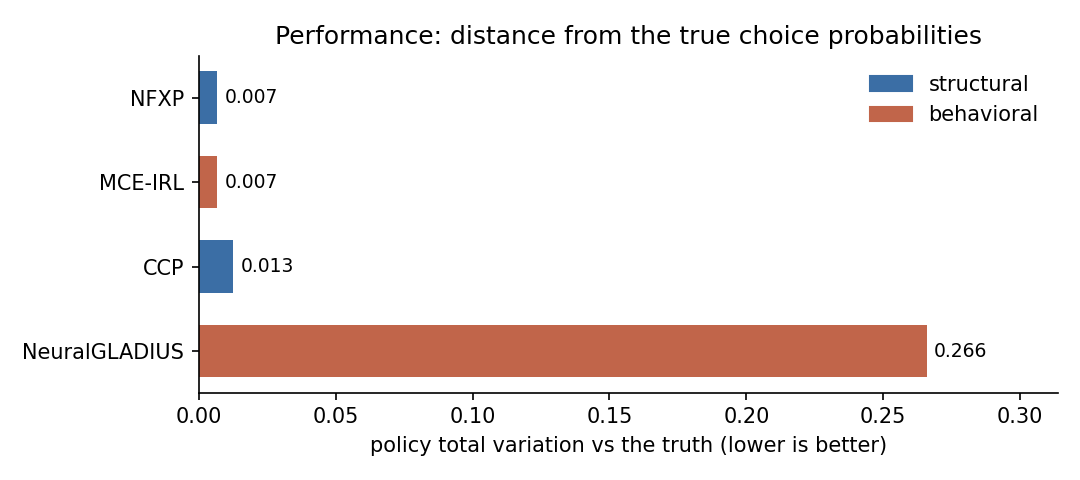
Param RMSE covers the structural family only, which shares the parameterization of the true model. Policy TV is the distance between estimated and true choice probabilities, lower is better. Conv is the estimator’s own convergence indicator. A cautious estimator can report False while the recovered policy is accurate. Regret base is welfare lost in the observed environment. Types A, B, and C are welfare lost after a change. Type A shifts a payoff, Type B changes the transitions, Type C penalizes an action. Estimators with a recovered reward re-solve it and adapt. Those without one keep their old policy.

Parameter recovery

Estimator	Parameter	True	Mean est	Bias	Emp. SE	RMSE	95% coverage	SE avail
NFXP	edge_cost	1.000	1.182	+0.182	0.083	0.191	1.00 +/- 0.00	100% (2 reps)
NFXP	amenity	0.500	0.508	+0.008	0.016	0.014	1.00 +/- 0.00	100% (2 reps)
NFXP	goal	1.000	0.999	-0.001	0.008	0.006	1.00 +/- 0.00	100% (2 reps)
CCP	edge_cost	1.000	1.167	+0.167	0.085	0.178	-	0% (2 reps)
CCP	amenity	0.500	0.488	-0.012	0.020	0.018	-	0% (2 reps)
CCP	goal	1.000	0.953	-0.047	0.018	0.049	-	0% (2 reps)

Coverage is the share of replications whose 95% interval contains the truth, shown with its Monte Carlo standard error. It is computed only where every replication produced a finite standard error. SE avail is the share of replications with finite standard errors.

The structural family (NFXP, CCP, MPEC) recovers all three parameters on the same scale as the truth, so Param RMSE applies to them alone. MCE-IRL here uses the same linear features and recovers the same values, but its weights stay out of the recovery table because an IRL reward is only partially identified in general. GLADIUS learns a neural policy object with no directly comparable reward weights in this study. Policy TV and regret are the right scorecards for the behavioral family.

Scaling

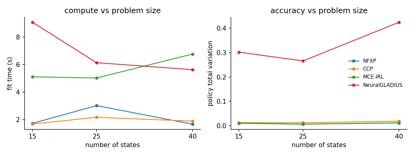
The same study at three problem sizes (15, 25, 40 states). Each line is one estimator: fit time on the left, policy total variation on the right. The structural methods stay accurate across sizes, with MPEC the fastest. GLADIUS is the least accurate at every size. The fits run from sub-second to a few seconds, so the compute lines reflect fixed overhead more than asymptotics at this scale.

Reward and structure

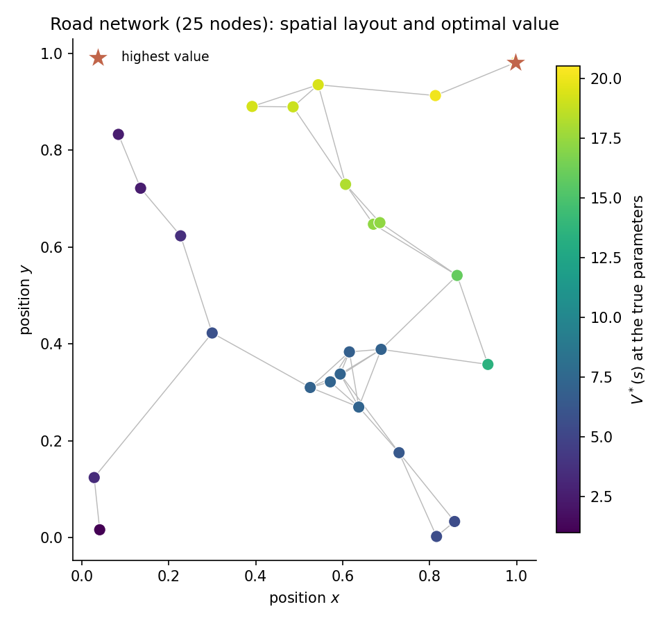
The network sits in the unit square. Each dot is a node, each line an edge. The color is the optimal value \(V^*(s)\) at the true parameters: value rises toward the goal node (the star). The spatial structure is the routing problem.

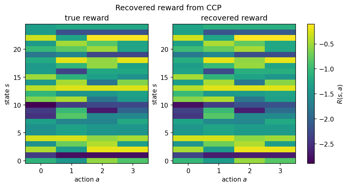
The recovered reward sits beside the true reward as state-by-action heatmaps, sharing one color scale. The recovered panel uses the best structural estimator’s mean coefficients. The two panels read the same, so the linear reward is recovered across the state space.

Notes per estimator

NFXP. Full-solution MLE with a nested Bellman fixed-point inner loop. Quadratic convergence near the optimum; all three parameters are identified from the edge-feature contrast.

CCP. CCP uses a first-step nonparametric policy estimate to avoid the inner Bellman loop. One policy-iteration step corrects the bias from the nonparametric first stage.

MCE-IRL. Its convergence indicator reports whether the gradient norm crossed the tolerance. The objective often plateaus before that, so it can read False while the recovered policy is accurate.

GLADIUS. Neural Q and continuation learner. Uses only the feature matrix and the observed panel; it does not use transition matrices in this study. Capped at 200 epochs here for short compute.

Reproduce

python scripts/study_route_choice.py                 # run + write JSON
python scripts/study_route_choice.py --page          # regenerate this page
python scripts/study_route_choice.py --verify        # re-derive the table from JSON

Results file: validation/results/study_route_choice.json.

Not shown on this page: MPEC, NNES, SEES, TD-CCP, and UFXP, because NFXP and CCP already cover the structural family on this small graph. IQ-Learn and f-IRL are omitted because reward is only partially identified from behavior here. Neural MCE-IRL, neural AIRL, and GLADIUS belong on larger or more reward-flexible studies.