MPEC

Mathematical programming with equilibrium constraints (MPEC) estimates the same structural dynamic discrete choice likelihood as NFXP, through a different numerical route. NFXP eliminates the value function by solving the Bellman fixed point inside every likelihood evaluation. MPEC keeps the value function as an explicit optimization variable and enforces the Bellman fixed point as an equality constraint. The reward parameters and the value vector are estimated jointly in a single constrained program.

Read this page as a numerical alternative to NFXP, not a different economic model. The target is the same likelihood; the risk is whether the constrained program is well conditioned enough to reach it.

Source Papers

The constrained formulation follows Su and Judd (2012). Iskhakov et al. (2016) compare the constrained and nested approaches and identify conditions under which the constrained problem degrades. The consistency argument follows Shapiro and Xu (2005). Finite-sample cautions for a related sequential-search MPEC estimator are reported in Koiso and Otani (2024).

Notation

Throughout, \(s \in \{1, \dots, S\}\) indexes the discrete state (\(S\) the total state count) and \(a\) the discrete action, observed for individual \(i\) in period \(t\). The vector \(\phi(s, a)\) collects the known reward features and \(\theta \in \mathbb{R}^K\) the reward parameters to be estimated (\(K\) the parameter dimension). The discount factor is \(\beta\) and the logit shock scale is \(\sigma\). The transition kernel \(P_a(s, s')\) gives the probability of moving to \(s'\) from \(s\) under action \(a\), stored in \((A, S, S)\) orientation. The value function is \(V\), held as an explicit variable in the constrained program. The choice-specific value is \(Q_\theta(s, a; V)\), which depends on the current value vector. The conditional choice probability, the policy, is \(\pi_{\theta, V}(a \mid s)\).

Model

The observed data are state, action, and next-state trajectories \((s_{it}, a_{it}, s_{i,t+1})\). The flow payoff is linear in the features:

\[ u_\theta(s, a) = \phi(s, a)^\top \theta. \]

With discount factor \(\beta\) and logit shock scale \(\sigma\), the soft Bellman operator maps a value vector to its log-sum-exp:

\[ T_\theta V(s) = \sigma \log \sum_a \exp\!\left( \frac{u_\theta(s, a) + \beta \sum_{s'} P_a(s, s') V(s')}{\sigma} \right). \]

The log-sum-exp form follows because integrating over Type-I extreme value shocks yields \(E[\max_a (Q_a + \varepsilon_a)] = \sigma \log \sum_a \exp(Q_a/\sigma)\) (standard result; see Rust 1987, Section 3).

Given a value vector \(V\), the choice-specific value is:

\[ Q_\theta(s, a; V) = u_\theta(s, a) + \beta \sum_{s'} P_a(s, s') V(s'). \]

The implied conditional choice probability follows the logit rule:

\[ \pi_{\theta, V}(a \mid s) = \frac{\exp(Q_\theta(s, a; V) / \sigma)} {\sum_b \exp(Q_\theta(s, b; V) / \sigma)}. \]

The canonical instance is Rust’s bus-engine replacement model. A bus operator decides each period whether to keep a deteriorating engine or pay a flat cost to replace it. The dynamic program links today’s choices to tomorrow’s states, so observed choices carry information about the structural costs.

Identification

This is the section that says when the constrained program has the same structural interpretation as NFXP rather than just a feasible optimizer output.

MPEC point-identifies the reward parameters \(\theta\) under the following assumptions, which are the same structural requirements as NFXP plus one additional condition arising from the constrained formulation.

Conditional independence (CI). The observed state transition is Markov in the current state and action and does not depend on the current logit shock.
Additive separability (AS). The per-period payoff is the systematic reward plus an additive choice-specific shock, drawn independently across choices as Type-I extreme value with fixed scale \(\sigma\).
Exogenous transitions. The transition kernel \(P_a(s, s')\) is supplied or estimated in a first stage, outside the payoff likelihood.
Reward normalization. The reward level and scale need an anchor. An exit or absorbing action with payoff fixed to zero pins the level, and the logit scale \(\sigma\) is held fixed.
Action-dependent feature rank. The reward features must vary across actions. The feature rank must equal the number of parameters. State-only features copied across actions collapse the action contrasts and leave \(\theta\) unidentified.
Constraint qualification. The Bellman constraint Jacobian must be numerically well-conditioned at the solution. A poorly conditioned Jacobian makes the equality-constrained program ill-posed even when the structural identification conditions hold.
State coverage. Each state must appear in the observed data. Unvisited states contribute no likelihood information to the corresponding Bellman constraint rows and can leave the constrained program ill-supported in those directions. The canonical tabular validation observes every state.

These hold inside a finite discrete state space, a stationary environment with expected-utility maximization, and a known, fixed discount factor \(\beta\). Given them, \(\theta\) is point-identified. Identification weakens under thin action support, an invalid normalization, a state space large enough that the Bellman constraint dimension strains the optimizer, or a discount factor approaching one.

Estimator

MPEC maximizes the conditional log likelihood jointly over the reward parameters and the value vector, subject to the Bellman equality constraint:

\[ (\hat\theta, \hat V) = \arg\max_{\theta,\, V}\ \sum_{i,t} \log \pi_{\theta, V}(a_{it} \mid s_{it}) \quad \text{subject to} \quad V - T_\theta V = 0. \]

At any feasible point the constraint forces \(V = V_\theta\), so MPEC and NFXP evaluate the same likelihood and target the same maximum likelihood estimate. When \(V = T_\theta V\), the choice-specific values \(Q_\theta(s, a; V)\) equal the Bellman Q-values, so \(\pi_{\theta, V}(a \mid s) = \pi_\theta(a \mid s)\); the two likelihoods are identical. The difference is numerical route, not structural object.

Standard errors use the same implicit-score identity as NFXP. At the constrained optimum, the sensitivity of the value function to the reward parameters satisfies:

\[ (I - \beta P_\pi)\, \frac{\partial V}{\partial \theta} = \sum_a \pi(a \mid s)\, \phi(s, a), \]

where \(P_\pi = \sum_a \operatorname{diag}(\pi_{\theta,V}(\cdot \mid a)) P_a\) is the policy-weighted transition matrix, with \(\operatorname{diag}(\pi_{\theta,V}(\cdot \mid a))\) denoting the \(S \times S\) diagonal matrix whose \((s,s)\) entry is \(\pi_{\theta,V}(a \mid s)\). Here \(\partial V / \partial \theta\) is an \(S \times K\) matrix; the linear system is solved once per reward parameter (\(K\) right-hand sides).

This equation follows from differentiating the Bellman fixed-point constraint \(V = T_\theta V\) totally with respect to \(\theta\):

\[ \frac{\partial V}{\partial \theta} = \frac{\partial (T_\theta V)}{\partial V}\,\frac{\partial V}{\partial \theta} + \frac{\partial (T_\theta V)}{\partial \theta}. \]

The two partial derivatives on the right are obtained from the log-sum-exp expression for \(T_\theta V(s)\):

Jacobian \(\partial (T_\theta V)/\partial V\). Differentiating \(\sigma \log \sum_a \exp(Q_\theta(s,a;V)/\sigma)\) with respect to \(V_{s'}\) gives \(\sum_a \pi(a \mid s)\, \beta P_a(s, s')\), so the \(S \times S\) Jacobian is \(\beta P_\pi\).
Feature gradient \(\partial (T_\theta V)/\partial \theta\). Differentiating with respect to \(\theta\) gives \(\sum_a \pi(a \mid s)\, \phi(s, a)\), the policy-weighted feature average.

Substituting both and rearranging yields \((I - \beta P_\pi)\,\partial V/\partial \theta = \sum_a \pi(a \mid s)\, \phi(s, a)\).

The per-observation score is obtained by the chain rule through \(\log \pi_{\theta,V}(a_{it} \mid s_{it})\):

\[ \frac{\partial \log \pi(a_{it} \mid s_{it})}{\partial \theta} = \frac{1}{\sigma}\!\left[ \phi(s_{it}, a_{it}) - \sum_b \pi(b \mid s_{it})\, \phi(s_{it}, b) \right] + \frac{\beta}{\sigma} \sum_{s'}\!\left[ P_{a_{it}}(s_{it}, s') - \sum_b \pi(b \mid s_{it})\, P_b(s_{it}, s') \right] \left(\frac{\partial V}{\partial \theta}\right)_{s'}, \]

where the second term uses the solved \(\partial V/\partial \theta\) from the linear system above. Stacking scores over observations, the sandwich covariance is \(\bigl(\sum_i g_i g_i^\top\bigr)^{-1}\) where \(g_i = \sum_t (\text{score at observation } it)\) is the per-individual score vector.

Shapiro and Xu (2005) establish that stationary points of the sample constrained problem converge to stationary points of the population problem (their Prop. 4.2), and that a sharp local optimum of the population problem is a sharp local optimum of the sample problem with probability approaching one (their Thm 5.4). Thm 5.4 is the hook into the standard delta-method / sandwich asymptotic normality result for smooth M-estimators: once the sample optimum tracks a unique, sharp population optimum, a Taylor expansion of the first-order conditions around the true parameter value yields \(\sqrt{N}(\hat\theta - \theta_0) \xrightarrow{d} N(0, J^{-1} \Sigma J^{-\top})\), where \(J\) is the population Hessian of the log-likelihood and \(\Sigma\) is the outer product of the score, the standard sandwich form for a smooth M-estimator. Shapiro and Xu supply the stochastic-MPEC analogue of the regularity conditions (their smoothing assumption and Lipschitz continuity of the equilibrium operator) that make the expected log-likelihood continuously differentiable in \(\theta\). Together these results justify treating the MPEC estimate as consistent and asymptotically normal under a well-specified tabular DDC with the assumptions above.

Algorithm

Algorithm  MPEC (constrained maximum likelihood, default solver="sqp")
Input   panel {(s_it, a_it, s_{i,t+1})}, features phi, transitions P,
        discount beta, logit scale sigma
Output  theta_hat, V_hat, standard errors, policy pi

 initialize theta
 solve  V_0 = T_theta V_0                      # warm start: Bellman fixed point
 form the joint variable  x = (theta, V)
 define equality constraint  c(x) = V - T_theta V   # one row per state
 repeat                                         # SQP outer loop (scipy SLSQP)
     compute  u(s, a) := phi(s, a)' theta
     compute  Q(s, a; V) := u(s, a) + beta * sum_{s'} P_a(s,s') V(s')
     compute  pi(a | s) := softmax(Q(s, :) / sigma)
     L(theta, V) := sum_{i,t} log pi(a_it | s_it)
    evaluate  c(x) and its Jacobian via JAX automatic differentiation
    update  x := (theta, V) via SQP step solving the quadratic subproblem
until the KKT stationarity norm and constraint violation fall below tolerance
check  |V - T_theta V|_inf                     # inspect final Bellman residual
solve  (I - beta P_pi) dV/dtheta = sum_a pi(a|s) phi(s,a)
compute per-observation scores and the robust covariance
return theta_hat, V_hat, standard errors, pi(theta_hat, V_hat)

The default solver is MPECConfig(solver="sqp"): scipy SLSQP solves the equality-constrained problem at each SQP step, with the objective gradient and the Bellman constraint Jacobian supplied by JAX. The value vector is initialized at the Bellman fixed point of the starting \(\theta\), so the optimizer begins feasible. No Bellman fixed-point solve is nested inside the likelihood objective.

Two additional variants are available. solver="sqp_jax" is an experimental JAX-native reduced-space SQP: it maintains \(V\) on the Bellman manifold by Newton-Kantorovich restoration steps and optimizes in \(\theta\)-space only using BFGS with an implicit-function-theorem gradient; it is slower than the default and intended for research comparison. solver="augmented_lagrangian" converts the constrained problem into a sequence of unconstrained L-BFGS-B subproblems with an increasing penalty on constraint violation; it is less reliable at discount factors near one. The string "slsqp" is a deprecated alias for "augmented_lagrangian", not scipy SLSQP; it emits a deprecation warning and its convergence indicator checks only Bellman feasibility, not optimality.

Applicability

Applicable when	Prefer an alternative when
States and actions are discrete.	The Bellman constraint is too large for a constrained optimizer.
Transitions are known or can be estimated first.	Transition estimation is the main modeling problem.
The reward has a compact parametric form.	The reward must be high-dimensional or neural.
Bellman constraint diagnostics are central.	Only the fastest repeated comparison run is needed.
A constrained-likelihood cross-check on NFXP is needed.	Only a behavioral cloning baseline is required.

MPEC targets the same structural object as NFXP and CCP through a different numerical route. CCP is usually faster when first-stage choice probabilities are well supported. NFXP nests the Bellman solve inside the likelihood and avoids the constraint-dimension scaling problem; Iskhakov et al. (2016) show the constrained problem can degrade as the state space grows or the discount factor approaches one. NNES and TD-CCP become attractive when the state space is too large for either repeated nested Bellman solves or the constrained program.

Usage

The public MPEC surface is the full estimator API. Create an estimator, call estimate, and inspect the returned summary:

from econirl.environments.rust_bus import RustBusEnvironment
from econirl.estimation.mpec import MPECEstimator, MPECConfig
from econirl.preferences.linear import LinearUtility
from econirl.simulation import simulate_panel

env = RustBusEnvironment(num_mileage_bins=20, discount_factor=0.99)
panel = simulate_panel(env, n_individuals=100, n_periods=50)
utility = LinearUtility.from_environment(env)

model = MPECEstimator(config=MPECConfig(solver="sqp"))
summary = model.estimate(
    panel=panel,
    utility=utility,
    problem=env.problem_spec,
    transitions=env.transition_matrices,
)

print(summary.parameters)
print(summary.metadata["final_constraint_violation"])

Inspect the Bellman residual before treating the result as structural evidence. A high likelihood with a large residual is not a solution:

# Check the Bellman residual at the solution.
violation = summary.metadata["final_constraint_violation"]
print(f"Bellman residual (inf-norm): {violation:.2e}")

# Read the policy at specific states.
print(summary.policy[[0, 5, 10, 19], :])

The Quick Start page documents the full set of fitted attributes and advanced API options.

Evidence

Parameter recovery is measured on a synthetic benchmark with known rewards, transitions, policies, values, Q functions, and Type A, Type B, and Type C counterfactual oracles. The figure below is a Monte-Carlo study: the panel is resimulated and refit on a fresh seed each time, and each parameter is plotted as its recovered mean and 95% interval against the true value.

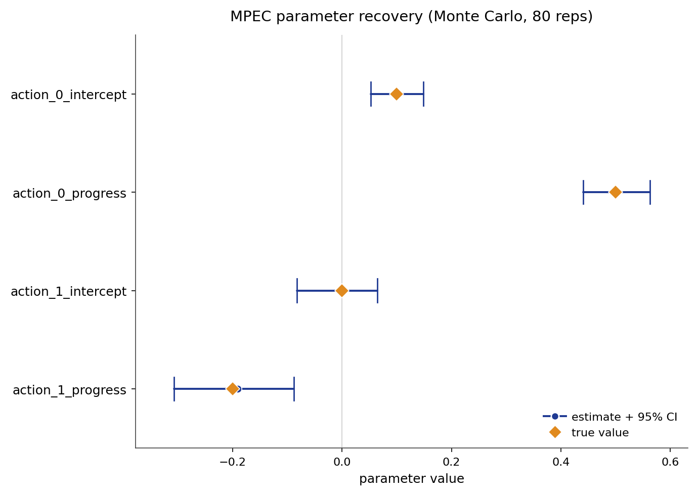
MPEC parameter recovery, Monte Carlo

Recovery is measured over a Monte-Carlo run of 80 replications.

Parameter	True	Recovered (mean)	95% interval
`action_0_intercept`	0.10	0.103	[0.053, 0.148]
`action_0_progress`	0.50	0.495	[0.441, 0.562]
`action_1_intercept`	0.00	-0.005	[-0.083, 0.064]
`action_1_progress`	-0.20	-0.190	[-0.307, -0.089]

Across the 80 replications the true value sits inside the 95% interval for every parameter, and the mean estimate is close to the truth.

The behavioral and regret numbers below were produced with solver="slsqp" (the legacy augmented-Lagrangian solver); the Algorithm section’s default and recommended solver is solver="sqp".

Behavioral fit and counterfactual regret on the same cell, against the known oracle objects:

Metric	Value
Policy total variation	0.0057
Value RMSE	0.0194
Type A regret (reward shift)	0.000213
Type B regret (transition change)	0.000362
Type C regret (action removed)	0.000086

The regrets are small because the recovered reward is close to the true reward and re-solving the intervened model reproduces nearly the same policy as the oracle. For the full cross-estimator comparison on the bus-engine panel, see the bus engine simulation study.

References

Source papers:

Su, C.-L. and Judd, K. L. (2012). Constrained Optimization Approaches to Estimation of Structural Models. Econometrica, 80(5), 2213-2230. reference entry.
Iskhakov, F., Lee, J., Rust, J., Schjerning, B., and Seo, K. (2016). Comment on “Constrained Optimization Approaches to Estimation of Structural Models.” Econometrica, 84(1), 365-370. reference entry.
Shapiro, A. and Xu, H. (2005). Stochastic Mathematical Programs with Equilibrium Constraints, Modeling and Sample Average Approximation. Optimization, 57(3), 395-418 (published 2008). reference entry.
Koiso, S. and Otani, S. (2024). An MPEC Estimator for the Sequential Search Model. arXiv:2409.04378. reference entry.

Implementation and reproduction:

Estimator source: econirl.estimation.mpec.
Validation runner: validation/estimators/mpec/run.py.
Results file: mpec.json.

Pages: