NNES
NNES (Neural Network Estimation of Structural models) is a structural dynamic discrete choice estimator that recovers finite-dimensional reward parameters while representing the continuation value with a trained neural network. The estimator embeds this approximation inside a nested pseudo-likelihood policy-iteration loop: at the true conditional choice probabilities, value-approximation errors are Neyman-orthogonal to the structural score, so the pseudo-likelihood Hessian is the correct variance estimator despite the neural nuisance object. The structural estimate supports counterfactual policy analysis; the neural network approximates the continuation value, not the reward.
Read this page carefully because the word “neural” does not mean the reward is neural. NNES keeps a finite structural reward target and uses the network as a continuation-value nuisance approximation.
Source Papers
The estimator follows Nguyen (2025), which introduces neural value approximation for structural dynamic discrete choice estimation and establishes the Neyman-orthogonality property of the nested pseudo-likelihood mapping. Hotz and Miller (1993) supply the conditional-choice-probability inversion underlying the profiled NPL step, and Aguirregabiria and Mira (2002) develop the nested pseudo-likelihood policy-iteration framework on which NNES builds.
Notation
Throughout, \(s\) indexes the discrete state and \(a\) the discrete action, observed for individual \(i\) in period \(t\). The vector \(\phi(s, a)\) collects the known reward features and \(\theta\) the finite-dimensional reward parameters to be estimated. The discount factor is \(\beta\) and the logit shock scale is \(\sigma\). The transition kernel \(P_a(s, s')\) gives the probability of moving to \(s'\) from \(s\) under action \(a\), stored in \((A, S, S)\) orientation. The integrated value function is \(V_\theta(s)\), its neural approximation is \(V_\psi(s)\) with network parameters \(\psi\), and the choice-specific value under the approximation is \(Q_{\theta,\psi}(s, a)\). The conditional choice probability, the policy, is \(\pi_{\theta,\psi}(a \mid s)\). The NPL policy iterate is \(\hat{P}(a \mid s)\). The dummy action index \(b\) ranges over the same action set as \(a\) and appears in softmax denominators.
The profiled integrated value \(W_\theta(\hat{P})\) is the solution to the policy-evaluation equation at fixed CCPs \(\hat{P}\); it equals \(V_\theta\) when \(\hat{P}\) coincides with the structural policy \(\pi_{\theta,\psi}\). The profiled value components \(W_z(\hat{P})\) and \(W_e(\hat{P})\) are defined by
where \(F_\pi[s,t] = \sum_a \hat{P}(a \mid s)\,P_a(s,t)\) is the transition matrix induced by the fixed CCP iterate, \(b_z[s,k] = \sum_a \hat{P}(a \mid s)\,\phi(s,a,k)\) is the policy-weighted feature vector, and \(b_e[s] = \sigma\,H\!\left(\hat{P}(\cdot \mid s)\right)\) is \(\sigma\) times the Shannon entropy at state \(s\):
Model
The observed data are state, action, and next-state trajectories \((s_{it}, a_{it}, s_{i,t+1})\). The flow payoff is linear in the features:
The integrated value function satisfies the soft Bellman fixed point:
NNES replaces the exact value object with a trained ReLU network \(V_\psi(s) \approx V_\theta(s)\), anchored so that \(V_\psi(s_0) = 0\) for a fixed anchor state \(s_0\). The choice-specific value under the approximation is:
The implied conditional choice probability follows the logit rule, where \(b\) runs over all actions in the denominator:
When \(V_\psi = V_\theta\), the choice-specific value recovers the Bellman-consistent \(Q\)-function and \(\pi_{\theta,\psi}\) coincides with the structural policy.
Connection to the linear system. The soft Bellman fixed point implies a policy-evaluation identity (Aguirregabiria and Mira 2002, logit social-surplus form): at the structural policy \(\hat{P} = \pi_\theta\), the expected integrated value satisfies
where \(H(s) = -\sum_a \hat{P}(a \mid s)\log\hat{P}(a \mid s)\) is the Shannon entropy of \(\hat{P}(\cdot \mid s)\). Substituting \(Q_{\theta,\hat{P}}(s,a) = u_\theta(s,a) + \beta\sum_{s'} P_a(s,s')\,V_\theta(s')\), writing \(u_\theta = \phi^\top\theta\), and rearranging yields the linear system
where \(b_z[s,k] = \sum_a \hat{P}(a\mid s)\phi(s,a,k)\) and \(b_e[s] = \sigma H(s)\). The linear system defines \(W_\theta\) by policy evaluation at the current CCP \(\hat{P}\); it equals the structural value \(V_\theta\) only when \(\hat{P} = \pi_\theta\), and approaches it as the NPL iterates converge. Because the right-hand side is affine in \(\theta\), the solution splits as \(W_\theta = W_z\theta + W_e\) via a single matrix solve.
The primary package evidence uses a high-action synthetic benchmark with 81 states (80 regular, 1 absorbing), a 16-dimensional encoded state representation, 3 actions, and 32 reward parameters. This cell tests whether the NPL-profiled neural value path recovers a finite-dimensional structural reward when the state representation is richer than a small tabular reference.
Identification
This is the section that says when the finite reward parameters remain interpretable even though a neural network enters the continuation value.
NNES point-identifies the reward parameters \(\theta\) under the following assumptions.
Conditional independence (CI). The observed state transition is Markov in the current state and action and does not depend on the current logit shock. This separates the transition dynamics from the payoff.
Additive separability (AS). The per-period payoff is the systematic reward plus an additive choice-specific shock, drawn independently across choices as Type-I extreme value with fixed scale \(\sigma\). The paper’s NPL orthogonality result is stated for this logit DDC structure.
Exogenous transitions. The transition kernel \(P_a(s, s')\) is supplied or estimated in a first stage, outside the payoff likelihood. NNES is model-based; without an available transition law, a transition-free estimator is required.
Reward normalization. The reward level and scale need an anchor. An absorbing or exit action with payoff fixed to zero pins the level, and the logit scale \(\sigma\) is held fixed.
Action-dependent feature rank. The reward features must vary across actions. The feature rank must equal the number of parameters; state-only features copied across actions collapse the action contrasts and leave \(\theta\) unidentified.
NPL Neyman-orthogonality. At the true conditional choice probabilities, first-order errors in the value approximation \(V_\psi\) drop out of the NPL structural score. Formally,
\[ \frac{\partial}{\partial \delta} \left[ \sum_i \frac{\partial \log \pi_{\theta,\, V_\psi + \delta}(a_i \mid s_i)} {\partial \theta} \right]_{\delta=0,\; \hat{P}=\pi_{\rm true}} = 0, \]where \(\delta\) represents a first-order perturbation to \(V_\psi\) (Nguyen 2025, Propositions 3-4). This zero-Jacobian / Neyman-orthogonality property means the pseudo-likelihood Hessian is the correct semiparametrically efficient variance estimator without an explicit debiasing correction.
Value-approximation regularity. The value-network approximation error must be small enough to enter the structural score only at second order. This is an asymptotic fourth-root-style requirement, not a finite-sample guarantee; a poor-fitting value network can contaminate recovery even when the data likelihood looks acceptable.
These hold inside a finite discrete state space, a stationary environment with expected-utility maximization, and a known, fixed discount factor \(\beta\). Identification weakens under thin action support, an invalid normalization, or a misoriented transition tensor. An unanchored value network can drift in high-discount problems because the absolute value level is weakly identified by choice data alone.
Estimator
For a fixed NPL policy iterate \(\hat{P}\), the policy-evaluation equation under the fixed CCPs is the linear system
where \(F_\pi[s,t] = \sum_a \hat{P}(a \mid s)\,P_a(s,t)\), \(b_z[s,k] = \sum_a \hat{P}(a \mid s)\,\phi(s,a,k)\), and \(b_e[s] = \sigma\,H(\hat{P}(\cdot \mid s))\) are as defined in the Notation block. Because the flow payoff \(u_\theta(s,a) = \phi(s,a)^\top\theta\) is linear in \(\theta\), the right-hand side is affine in \(\theta\), so the solution splits by linearity of the matrix solve:
This affine structure is what makes NPL profiling possible: the value target is computed once per outer iteration by a single matrix solve, with no inner Bellman loop.
Differentiating \(W_\theta[\hat{P}] = W_z\,\theta + W_e\) with respect to \(\theta\) at fixed \(\hat{P}\) gives \(\partial W / \partial\theta = W_z\) (since \(W_z\) depends only on \(\hat{P}\) and the transitions, not on \(\theta\)). Substituting into the choice-specific value \(Q_{\theta,\psi}(s,a) = \phi(s,a)^\top\theta + \beta\sum_{s'} P_a(s,s')\,V_\psi(s')\), and replacing \(V_\psi\) with the profiled target \(W_\theta[\hat{P}]\), gives:
The profiled choice value is therefore \(Q^{\hat{P}}(s,a) = \tilde{z}(s,a)^\top\theta + \tilde{e}(s,a)\), where \(\tilde{z}(s,a) = \phi(s,a) + \beta\,\mathbb{E}[W_z(s') \mid s,a]\) and \(\tilde{e}(s,a) = \beta\,\mathbb{E}[W_e(s') \mid s,a]\). No Bellman fixed-point differentiation is needed; the implicit-differentiation analog \((I - \beta F_\pi)\,\partial W/\partial\theta = b_z\) is solved once via \(W_z\).
The value network \(V_\psi\) is trained by supervised regression on the profiled target \(W_\theta[\hat{P}]\), and the structural parameters are recovered by maximizing the profiled pseudo-likelihood over \(\tilde{z}\) and \(\tilde{e}\):
The outer optimizer is L-BFGS-B. After the maximization step, conditional choice probabilities are updated from the implied logit policy and the loop repeats. The per-observation score from this profiled pseudo-likelihood has the logit form:
where the gradient flows through \(W_z(\hat{P})\) rather than through the Bellman fixed point, so no inner-loop differentiation is required. The estimator solves \(\sum_{i,t} \ell_{it}'(\theta) = 0\), equivalently the argmax above.
Algorithm
Algorithm  NNES-NPL (neural nested pseudo-likelihood, default variant)
Input   panel {(s_it, a_it, s_{i,t+1})}, features phi, transitions P,
        discount beta, logit scale sigma, value network V_psi,
        outer iterations K
Output  theta_hat, policy pi, value approximation V_psi

1   initialize theta
2   initialize hat_P(a | s) from empirical state-action frequencies
3   repeat K times                          # outer NPL loop
4       W_z, W_e := profiled_value_components(hat_P, P, phi, beta, sigma)
5       target_V := W_z * theta + W_e       # value profiled as affine in theta
6       target_V := target_V - target_V[anchor_state]   # anchor normalization
7       train V_psi on target_V by supervised regression
8       Q(s, a) := phi(s, a)' theta + beta * sum_{s'} P_a(s, s') V_psi(s')
9       pi(a | s) := exp(Q(s, a)/sigma) / sum_b exp(Q(s, b)/sigma)
10      theta := argmax_theta sum_{i,t}
              log softmax((z_tilde(s_it,.) theta + e_tilde(s_it,.)) / sigma)[a_it]
              # uses Q^P_hat = z_tilde theta + e_tilde (profiled, not Bellman-fixed)
12      hat_P := pi                         # update policy iterate
13  return theta_hat, standard errors from the profiled Hessian, pi, V_psi
The default variant is bellman="npl" (the NNESEstimator class in
econirl.estimation.nnes). This is the path with the Neyman-orthogonality
property; standard errors from the profiled Hessian are semiparametrically
efficient. The alternative bellman="nfxp" invokes NNESNFXPEstimator, which
trains the value network to satisfy the NFXP soft-Bellman residual rather than
the NPL profiled target. This variant does not carry the orthogonality guarantee:
value-approximation errors enter the structural score directly, so standard errors
from its Hessian are not semiparametrically efficient. The "nfxp" variant is
available as a diagnostic but is not the reported inference path.
Applicability
Applicable when |
Prefer an alternative when |
|---|---|
States and actions are discrete. |
The state space is small enough for exact NFXP or tabular CCP. |
The reward is finite-dimensional and parametric. |
The reward itself must be unrestricted or neural. |
The value object is too large, encoded, or smooth for repeated exact Bellman solves. |
Transitions are unavailable; use TD-CCP or a transition-free estimator. |
Transitions are known or can be estimated first. |
Only in-sample choice probabilities are required. |
Counterfactual policy analysis under changed primitives is required. |
Only a fast imitation baseline is required. |
A flexible value approximation is the modeling objective. |
The cleanest exact-likelihood structural reference is required. |
NNES targets the same finite-dimensional structural object as NFXP, CCP, and MPEC, but replaces the exact tabular Bellman solve with a neural value approximation. CCP and MPEC use tabular continuation objects; SEES uses a deterministic basis-function sieve. NNES becomes attractive when encoded states or high-dimensional state representations make a neural value function the natural modeling choice. On small tabular problems, exact NFXP or CCP can still dominate because the neural training overhead exceeds the savings from avoiding exact dynamic programming.
Usage
from econirl.datasets import load_rust_bus
from econirl import NNES

df = load_rust_bus()

model = NNES(
    n_states=90,
    n_actions=2,
    discount=0.9999,
    utility="linear_cost",
    bellman="npl",
    hidden_dim=32,
    num_layers=2,
    v_epochs=500,
    n_outer_iterations=3,
)
model.fit(df, state="mileage_bin", action="replaced", id="bus_id")

print(model.params_)
print(model.summary())
The fitted policy gives action probabilities by state and can be read at specific states:
print(model.predict_proba([0, 20, 40, 60, 80])) # shape (5, n_actions)
Counterfactual policy analysis re-solves the structural model under changed
primitives using the simulation harness. The public wrapper does not expose a
counterfactual() method; the full NNESEstimator API is the route for
counterfactual re-solves in research workflows. The
Counterfactuals subpage documents the three
counterfactual types and the harness-level results.
The Quick Start page documents the full set of fitted
attributes and the full NNESEstimator API.
Evidence
Parameter recovery is measured on a high-action synthetic benchmark with 81 states, a 16-dimensional encoded state representation, 3 actions, and 32 reward parameters, with known oracle reward, policy, value, Q, and counterfactual objects. The figure below is a Monte-Carlo study over 25 replications: the panel is resimulated and refit on a fresh seed each time, and each parameter is plotted as its recovered mean and 95% interval against the true value.
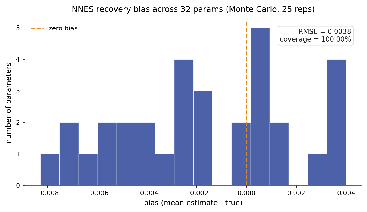
The recovery study resimulates and refits across 25 replications. The estimator recovers all 32 value-function weights: the aggregate recovery RMSE is 0.0038, and the true value falls inside the 95% interval for all 32 of 32 weights. The figure shows the per-weight recovery-error distribution.
Behavioral fit and counterfactual regret on the canonical_high_action primary
cell, against the known oracle objects from validation/results/nnes.json:
Metric |
Value |
|---|---|
Policy total variation |
0.0238 |
Value RMSE |
0.1156 |
Type A regret (reward shift) |
0.004865 |
Type B regret (transition change) |
0.005559 |
Type C regret (action removed) |
0.001314 |
All three regret values fall below the 0.05 threshold. The behavioral metrics are from a single-fit oracle-comparison run, not a Monte-Carlo average; they will be updated when the recovery study is complete. Current standard errors are not available in the results file; that entry remains pending the Monte-Carlo run. For the full cross-estimator comparison on the bus-engine panel, see the bus engine simulation study.
References
Source papers:
Nguyen, H. (2025). “Neural Networks for Efficient Estimation of High-Dimensional Dynamic Discrete Choice Models.” Working paper, Georgetown University. reference entry.
Hotz, V. J., and Miller, R. A. (1993). “Conditional Choice Probabilities and the Estimation of Dynamic Models.” Review of Economic Studies, 60(3), 497-529. reference entry.
Aguirregabiria, V., and Mira, P. (2002). “Swapping the Nested Fixed Point Algorithm: A Class of Estimators for Discrete Markov Decision Models.” Econometrica, 70(4), 1519-1543. reference entry.
Implementation and reproduction:
Estimator source:
econirl.estimation.nnes.sklearn wrapper:
econirl.NNES.Validation runner:
validation/estimators/nnes/run.py.Recovery study:
validation/estimators/nnes/recovery_mc.py(pending; adapt fromvalidation/estimators/nfxp/recovery_mc.py).Results file:
nnes.json.
Pages: