TD-CCP

TD-CCP estimates finite-dimensional structural reward parameters in dynamic discrete choice models using conditional choice probabilities and temporal-difference recursions. The parameter-estimation stage recovers the linear reward weight vector \(\theta\) without constructing a model for the transition density. Observed current and successor state-action pairs identify two recursive continuation objects, which enter a CCP pseudo-log-likelihood in place of the transition integral. Cross-fitted, locally robust standard errors correct for first-stage estimation error in those objects and deliver valid inference at parametric rates.

Read this page when the transition density is the obstacle. TD-CCP still targets finite structural reward parameters; it changes how recursive continuation terms are estimated.

Source Papers

The estimator follows Adusumilli and Eckardt (2025), which introduces the temporal-difference CCP construction, the semigradient closed-form solve for the continuation accumulators, the locally robust correction recursion, and a cross-fitting procedure for valid inference. The CCP foundation is Hotz and Miller (1993), which first expresses the dynamic programming problem in terms of conditional choice probabilities and inverts the CCP mapping to recover structural parameters.

Theory Connections

For the proof route behind this page, start with Identification and Anchors for the normalization problem and Classical DDC Estimators for how the CCP route replaces repeated Bellman solves with recursive continuation objects. Use Reward Projection and Feature Rank for the rank condition behind the projected parameter recovery step.

Notation

Throughout, \(x\) indexes the discrete state and \(a\) the discrete action, following the notation of Adusumilli and Eckardt (2025). Observations are recorded for individual \(i\) in period \(t\) as current and successor tuples \((a_t, x_t, a_{t+1}, x_{t+1})\). The vector \(z(a, x)\) collects the known reward features and \(\theta\) the finite-dimensional reward parameter vector. The discount factor is \(\beta\) and the logit shock scale is \(\sigma\). The transition kernel \(P_a(x, x')\) gives the probability of moving to \(x'\) from \(x\) under action \(a\), stored in \((A, S, S)\) orientation; the parameter-estimation stage does not model this kernel. The first-stage conditional choice probability is \(P(a \mid x)\). The reward-feature accumulator is \(h(a, x)\) and the choice-shock accumulator is \(g(a, x)\); both are identified from observed successor pairs without a density model. The basis function \(\phi(a, x)\) is a user-chosen finite-dimensional feature vector over (action, state) pairs that spans the approximation space for \(h\) and \(g\); the default is action-interacted polynomial functions of the state index; the estimated accumulator evaluates as \(\hat{h}(a, x) = \phi(a, x)^\top \hat{\omega}\). The integrated value function is \(V_\theta(x)\) and the choice-specific value is \(\tilde{Q}_\theta(a, x) = h(a, x)^\top \theta + g(a, x)\).

Model

The data are current and successor state-action tuples \((a_t, x_t, a_{t+1}, x_{t+1})\) from a stationary infinite-horizon discrete choice model. The flow payoff is linear in known reward features:

\[ u_\theta(a, x) = z(a, x)^\top \theta. \]

The reward-feature accumulator \(h\) satisfies the Bellman-style recursion:

\[ h(a, x) = z(a, x) + \beta\,\mathbb{E}\bigl[h(a', x') \mid a, x\bigr]. \]

The choice-shock accumulator \(g\) satisfies:

\[ g(a, x) = \beta\,\mathbb{E}\bigl[e(a', x') + g(a', x') \mid a, x\bigr], \qquad e(a, x) = \gamma_{\mathrm{E}} - \log P(a \mid x), \]

where \(\gamma_{\mathrm{E}}\) is the Euler-Mascheroni constant and \(e(a, x)\) is the CCP-inverted shock accumulator. Under the logit model, the expected shock conditional on choosing \(a\) is \(\mathbb{E}[\varepsilon_a \mid a \text{ chosen}] = \gamma_{\mathrm{E}} - \log \pi(a \mid x)\) (Hotz and Miller 1993), so \(e(a, x) = \gamma_{\mathrm{E}} - \log P(a \mid x)\) recovers the conditional shock from the observed CCP. Neither recursion requires modeling the transition density; both are identified from observed successor pairs.

Substituting the Bellman equation recursively, the choice-specific value \(Q(a, x)\) decomposes linearly into a reward-accumulator term \(h(a, x)^\top \theta\) and a choice-shock term \(g(a, x)\) that absorbs all future logit shocks (the Q-decomposition of Adusumilli and Eckardt 2025). This decomposition holds because the linear reward structure lets the two accumulators be estimated separately. The implied choice-specific value is:

\[ \tilde{Q}_\theta(a, x) = h(a, x)^\top \theta + g(a, x), \]

and the conditional choice probability follows the logit rule with scale \(\sigma\):

\[ \pi_\theta(a \mid x) = \frac{\exp\{\tilde{Q}_\theta(a, x) / \sigma\}} {\sum_b \exp\{\tilde{Q}_\theta(b, x) / \sigma\}}. \]

The implementation uses the full \(\sigma\) via problem.scale_parameter at every evaluation point; the default is \(\sigma = 1\).

The canonical evaluation instance is the encoded-state design: 81 states, 3 actions, and 6 reward parameters. Reward features are polynomial functions of two encoded state coordinates; action 0 serves as the reward-normalized baseline.

Identification

This is the section that says when successor tuples and CCPs are enough to recover the reward parameters without modeling the transition density.

TD-CCP point-identifies the reward parameters \(\theta\) under the following assumptions.

• Conditional Independence (CI). The observed state transition is Markov in the current state and action and does not depend on the current logit shock.

• Additive Separability (AS). The per-period payoff is the systematic reward plus an additive choice-specific shock, drawn independently across choices as Type-I extreme value with fixed scale \(\sigma\).

• Finite Linear Reward. The flow utility is a known finite-dimensional linear function \(z(a, x)^\top \theta\) of the reward features. The reward target is the finite parameter vector \(\theta\); the estimator does not recover an unrestricted functional form.

• Reward Normalization. A baseline action with reward features fixed to zero anchors the reward level and pins the logit scale.

• Action-Dependent Feature Rank. The reward features must vary across actions; the action-contrast rank must equal the number of parameters. State-only features copied identically across actions difference out of the choice probabilities and leave \(\theta\) on a ridge.

These hold in a finite discrete state space, a stationary environment, and with a known fixed discount factor \(\beta\). Given these conditions, \(\theta\) is point-identified. Identification weakens under thin action support (which destabilizes first-stage CCPs), an invalid reward normalization, or a near-singular basis for the continuation accumulators.

Estimator

The preliminary estimator maximizes the CCP pseudo-log-likelihood:

\[ \tilde{\theta} = \arg\max_\theta \sum_{i,t} \log \pi_\theta(a_{it} \mid x_{it}), \]

where \(\pi_\theta\) uses the semigradient estimates \(\hat{h}\) and \(\hat{g}\) in place of the transition integral. The basis function \(\phi(a, x)\) is a user-chosen finite-dimensional feature vector over (action, state) pairs that spans the approximation space for \(h\) and \(g\); the default is action-interacted polynomial functions of the state index. The semigradient solve for \(h\) takes the closed form:

\[ \hat{\omega} = \Bigl[\mathbb{E}_n\bigl\{\phi(a,x) \bigl(\phi(a,x) - \beta\phi(a',x')\bigr)^\top\bigr\}\Bigr]^{-1} \mathbb{E}_n\bigl\{\phi(a,x)\,z(a,x)\bigr\}, \]

with \(\hat{h}(a, x) = \phi(a, x)^\top \hat{\omega}\). The analogous equation for \(g\) substitutes the next-period shock \(\beta\, e(a', x')\) as the regression target:

\[ \hat{\omega}_g = \Bigl[\mathbb{E}_n\bigl\{\phi(a,x) \bigl(\phi(a,x) - \beta\phi(a',x')\bigr)^\top\bigr\}\Bigr]^{-1} \mathbb{E}_n\bigl\{\phi(a,x)\cdot \beta\, e(a', x')\bigr\}, \quad e(a, x) = \gamma_{\mathrm{E}} - \log P(a \mid x). \]

The matrix \(A = \mathbb{E}_n\{\phi(\phi - \beta\phi')^\top\}\) is shared between the \(h\) and \(g\) solves, so both require only one matrix inversion.

The score of the pseudo-log-likelihood with respect to \(\theta\) is:

\[ \frac{\partial}{\partial \theta} \log \pi_\theta(a \mid x) = \frac{h(a, x) - \sum_b \pi_\theta(b \mid x)\, h(b, x)}{\sigma}. \]

Setting \(\mathbb{E}_n[\text{score}] = 0\) and treating \(\hat{h}\) and \(\hat{g}\) as fixed gives the partial MLE first-order condition that defines \(\tilde{\theta}\).

Locally Robust Inference

The plug-in score ignores estimation error in \(\hat{h}\) and \(\hat{g}\). The locally robust correction debiases the moment by adding a term indexed by \(\lambda(a, x)\). The corrected moment for observation \(i\) is:

\[ \zeta_i = m_i + \lambda(a_i, x_i) \cdot \delta_i, \]

where \(m_i = \partial_\theta \log \pi_\theta(a_i \mid x_i)\) is the plug-in score and \(\delta_i\) collects the TD residuals of \(h\) and \(g\) at observation \(i\) (Adusumilli and Eckardt 2025). The correction function \(\lambda\) solves the backward fixed-point:

\[ \lambda(a', x') = -m(a', x';\,\theta,\hat{h},\hat{g}) + \beta\,\lambda(a, x), \]

reversing the time direction relative to the forward recursion for \(h\) and \(g\). Sign convention note. This page writes the correction moment as \(\zeta_i = m_i + \lambda \cdot \delta_i\) and the backward recursion with \(-m\). Adusumilli and Eckardt (2025) may use the opposite sign on \(m\) together with a compensating sign on \(\zeta\); the two conventions are algebraically equivalent and produce the same corrected estimator. The robust estimator \(\hat{\theta}\) solves \(\mathbb{E}_n[\zeta_i] = 0\). The asymptotic variance is given by the sandwich formula:

\[ \hat{V} = \bigl(G^\top \hat{\Omega}^{-1} G\bigr)^{-1}, \quad G = \mathbb{E}_n\!\left[\frac{\partial \zeta_i}{\partial \theta^\top}\right], \quad \hat{\Omega} = \mathbb{E}_n[\zeta_i \zeta_i^\top]. \]

Under the conditions of Adusumilli and Eckardt (2025), \(\sqrt{n}(\hat{\theta} - \theta_0) \to \mathcal{N}(0, V)\). With cross-fitting (the cross-fitting procedure of Adusumilli and Eckardt 2025), \(\lambda\) is computed on one fold using objects learned on the complementary fold, giving valid inference at parametric rates with standard errors clustered by individual. The deep asymptotic proof is stated and cited; it is not re-derived here.

Algorithm

Algorithm  TD-CCP (semigradient, locally robust cross-fitting)
Input   panel {(a_it, x_it, a_{i,t+1}, x_{i,t+1})}, reward features z,
        basis phi, discount beta, fold count K
Output  theta_hat, standard errors, policy pi, value V

1   estimate first-stage CCPs P(a | x) from observed choices          # logit or frequency
2   partition individuals into K folds
3   for k = 1, ..., K:
4       using data from folds != k, solve for h_k by semigradient TD:
            omega_k = [E_n{phi(a,x)(phi(a,x) - beta phi(a',x'))'}]^{-1}
                       E_n{phi(a,x) z(a,x)}
5       using data from folds != k, solve for g_k analogously
            with target beta (gamma_E - log P(a' | x'))
6       on fold k data, solve the preliminary CCP pseudo-likelihood for tilde_theta_k
7       on fold k data, compute the correction recursion lambda_k           # backward fixed-point; see Locally Robust Inference
8       on fold k data, solve the locally robust moment equation for theta_k # zeta_i = 0; see Locally Robust Inference
9   theta_hat := average_k(theta_k)
10  standard errors from the fold covariances, clustered by individual
11  return theta_hat, standard errors, policy pi_theta, value V_theta

The parameter-estimation stage does not model the transition kernel; the accumulators \(\hat{h}\) and \(\hat{g}\) are identified entirely from observed successor pairs \((a_t, x_t, a_{t+1}, x_{t+1})\).

The default estimator uses method="semigradient", cross_fitting=True, and robust_se=True, implementing the locally robust cross-fitting procedure of Adusumilli and Eckardt (2025). The semigradient steps (4 and 5) reduce to single matrix solves, making recursive-term estimation fast. The alternative method="neural" replaces the semigradient closed-form solves with neural approximate value iteration, which trains neural networks for \(h\) and \(g\) iteratively; it is more flexible for high-dimensional state spaces and does not use cross-fitting or locally robust standard errors in the current implementation.

System View

TD-CCP keeps the finite reward-parameter target but avoids estimating a full transition density during parameter estimation. It does this by learning the recursive continuation terms directly from observed successor state-action pairs.

Observed tuples: current action/state and next action/state
Reward features, first-stage choice probabilities, discount factor
        |
        v
Estimate continuation accumulators from successor pairs
        |
        v
Build a CCP pseudo-likelihood using those accumulators
        |
        v
Estimate finite reward parameters theta
        |
        v
Use a post-fit transition environment for policy, value,
and counterfactual evaluation

“Transition-density-free” describes the estimation step. It does not remove the economics of transitions, and it does not make counterfactuals possible without an environment to re-solve.

Applicability

Applicable when	Prefer an alternative when
Choices are discrete and agents are forward-looking.	The state space is small and tabular Bellman solves are feasible (NFXP).
The panel records current and next state-action pairs.	The panel does not record successor states or actions.
Transition-density modeling is the main bottleneck.	Transitions are known or easily estimated (CCP or NFXP).
The reward is a finite linear function of known features.	The reward target is an unrestricted neural map (IRL family).
Locally robust standard errors are required for inference.	Observed action support is very sparse at key states.

TD-CCP occupies the niche between exact tabular methods and IRL. NFXP and MPEC nest the Bellman solve inside the likelihood and require the full transition tensor; CCP inverts the CCP mapping and needs the transition object for the future-value terms. TD-CCP sidesteps the transition-density modeling step entirely for reward-parameter estimation, at the cost of requiring observed successor state-action pairs in the panel. NNES and UFXP are attractive when Bellman solves are feasible but the main goal is computation speed. Counterfactual evaluation under an intervened transition process still requires a transition environment; TD-CCP’s advantage is confined to the parameter-estimation stage.

Usage

from econirl.datasets import load_rust_bus
from econirl import TDCCP

df = load_rust_bus()

model = TDCCP(
    n_states=90,
    n_actions=2,
    discount=0.9999,
    utility="linear_cost",
    method="semigradient",
)
model.fit(df, state="mileage_bin", action="replaced", id="bus_id")

print(model.params_)
print(model.summary())

The fitted policy gives the action probability at each state:

states = [0, 10, 50, 89]
print(model.predict_proba(states))

Counterfactual evaluation re-solves the dynamic program under a changed reward or transition primitive. The public wrapper exposes the fitted parameters, policy, and confidence intervals; re-solution under an intervened environment uses econirl.estimation.td_ccp.TDCCPEstimator with a supplied transition tensor. See the Counterfactuals subpage for the counterfactual taxonomy and reported regret values.

The Quick Start page documents the full set of fitted attributes and the full TDCCPEstimator API.

Evidence

Parameter recovery is measured on a deliberately hard synthetic benchmark with encoded-state features and locally robust inference. It has known rewards, transitions, policies, values, Q functions, and Type A, Type B, and Type C counterfactual oracles. The figure below is a Monte-Carlo study: the panel is resimulated on a fresh seed each replication, and each parameter is plotted as its recovered mean and 95% interval against the true value.

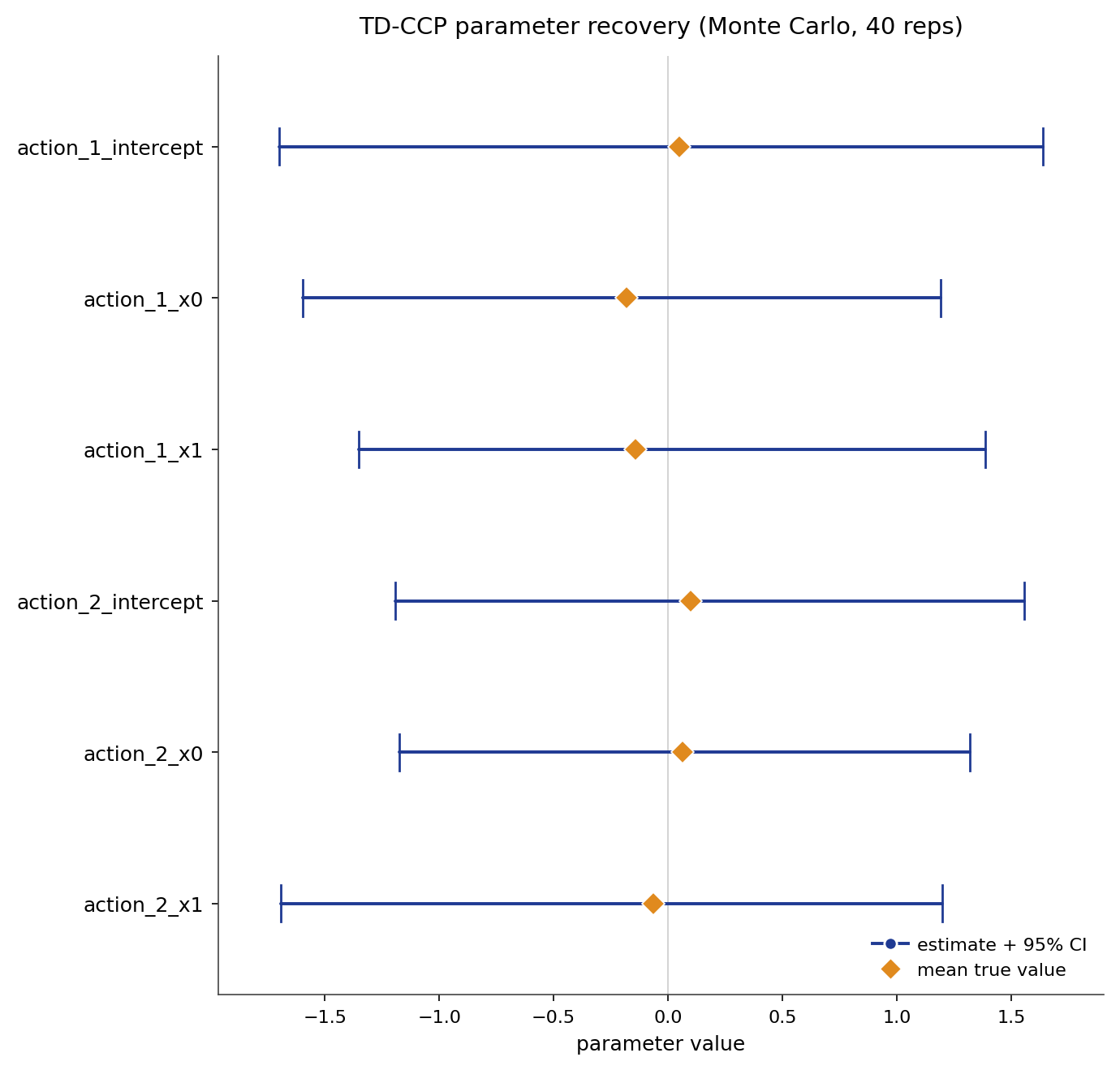
Parameter recovery on the encoded-state benchmark across 40 replications. Each replication resimulates the panel on a fresh seed and refits the estimator.

Parameter	True	Recovered (mean)	95% interval
action_1_intercept	0.048	0.039	[-1.700, 1.638]
action_1_x0	-0.182	-0.170	[-1.598, 1.194]
action_1_x1	-0.144	-0.137	[-1.352, 1.388]
action_2_intercept	0.100	0.096	[-1.194, 1.558]
action_2_x0	0.065	0.076	[-1.174, 1.320]
action_2_x1	-0.063	-0.068	[-1.693, 1.198]

The mean estimate recovers each parameter, but the deliberately hard case has high per-replication variance, so the 95% intervals are wide. The width reflects finite-sample difficulty, not bias.

Behavioral fit and counterfactual regret on the same cell, against the known oracle objects:

Metric	Value
Policy total variation	0.004658
Value RMSE	0.020109
Type A regret (reward shift)	0.001883
Type B regret (transition change)	0.001864
Type C regret (action removed)	0.003200

The regrets are small because the recovered reward is close enough to the truth that re-solving under the intervened primitive reproduces almost the same policy as the oracle. For the full cross-estimator comparison on a bus-engine panel, see the bus engine simulation study.

References

Source papers:

• Adusumilli, K., and Eckardt, D. (2025). “Temporal-Difference Estimation of Dynamic Discrete Choice Models.” Working paper. reference entry.

• Hotz, V. J., and Miller, R. A. (1993). “Conditional Choice Probabilities and the Estimation of Dynamic Models.” Review of Economic Studies, 60(3), 497-529. reference entry.

Implementation and reproduction:

• Estimator source: econirl.estimation.td_ccp.

• sklearn wrapper: econirl.TDCCP.

• Validation runner: validation/estimators/tdccp/run.py.

• Results file: tdccp.json.

Pages:

• Quick Start

• Pre-Estimation Checks

• Simulation Study

• Counterfactuals

• Rust Bus Engine Example