Direct optimization approaches

Most structural estimators of dynamic discrete choice nest a Bellman fixed-point solve inside every optimization step: NFXP and Deep MCE-IRL re-solve for the value function each time the reward parameters change. Direct optimization avoids the inner loop. It lifts the value function into the optimizer as a free variable and solves a single problem, imposing the Bellman equation as a constraint rather than re-deriving it. Three estimators are compared here, all on the same anchored data. Tabular MPEC carries a linear reward and a value vector and imposes the soft Bellman equation as a hard equality. Neural MPEC replaces both with networks, so the equality relaxes to a soft penalty over a state grid. GLADIUS drops the known transitions entirely and learns an expected-value network in their place.

The three estimators

The setting is a finite MDP with states \(s\), actions \(a\), discount \(\beta=0.95\), and logit scale \(\sigma=1\). The choice-specific value is

\[ Q(s,a) = u(s,a) + \beta \sum_{s'} P_a(s,s')\,V(s'), \]

the logit policy is \(\pi(a\mid s) = \mathrm{softmax}_a\!\big(Q(s,\cdot)/\sigma\big)\), and the soft Bellman operator is

\[ TV(s) = \sigma \log \sum_a \exp\!\big(Q(s,a)/\sigma\big). \]

At a solution \(V = TV\). The three methods differ in how the reward is parameterized, whether \(P_a(s,s')\) is known, and how the Bellman condition enters the optimization.

Tabular MPEC (Su and Judd, 2012) uses a linear reward \(u_\theta(s,a) = \phi(s,a)^\top \theta\) and known transitions. It treats the value vector \(V\) as a free variable alongside \(\theta\) and imposes the soft Bellman equation as a hard equality constraint, solved by SLSQP:

\[ \max_{\theta,\,V} \ \sum_{it} \log \pi_{\theta,V}(a_{it}\mid s_{it}) \quad \text{s.t.} \quad V - TV = 0. \]

Because \(V\) is a finite vector, the constraint can be enforced exactly at every state.

Neural MPEC replaces the linear reward with a network \(u_\theta(s,a)\) and the value vector with a network \(V_\phi(s)\), keeping the transitions known. Once \(V\) is a network it cannot satisfy a hard equality at every state, so the Bellman condition becomes a soft penalty evaluated at a set of collocation points (here the full state grid). The loss is

\[ -\frac{1}{N}\sum_{it} \log \pi(a_{it}\mid s_{it}) \;+\; \frac{\rho}{2} \sum_{s} w(s)\,\big(V_\phi(s) - TV(s)\big)^2 . \]

Because \(P_a(s,s')\) is known, the expectation \(\sum_{s'} P_a(s,s')\,V_\phi(s')\) is a matrix-vector product computed exactly, with no double-sampling of transitions. The reward is anchored so that the reference action carries zero utility, \(u_\theta(s,2) \equiv 0\). The co-training step is short:

def loss_fn(m, rho_):
    u_all = m.reward.all_actions(onehot)
    V_all = m.value.all_states(onehot)
    EV = jnp.einsum("ast,t->as", T, V_all)
    Q = u_all + BETA * EV.T
    logp = jax.nn.log_softmax(Q / SIGMA, axis=1)
    nll = -logp[obs_s, obs_a].mean()
    resid = V_all - SIGMA * jax.scipy.special.logsumexp(Q / SIGMA, axis=1)
    return nll + 0.5 * rho_ * jnp.sum(w * resid**2), None

The einsum is the exact expected continuation value; resid is the per-state Bellman residual that the penalty drives toward zero.

GLADIUS is model-free. It carries a neural \(Q\) network and a neural expected-value (EV) network and trains them single-loop with a soft Bellman consistency penalty applied to observed transitions. It never uses \(P_a(s,s')\): the EV network stands in for \(\sum_{s'} P_a(s,s')\,V(s')\) and is learned from data. It is run here at the repository-standard network size (128 wide, 3 layers, 500 epochs) with the same action-2 anchor the MPEC methods receive, so it is a fair model-free baseline. Because it does not use the transitions, its recovered reward is in a different parameterization than the known-\(P\) methods.

Setup

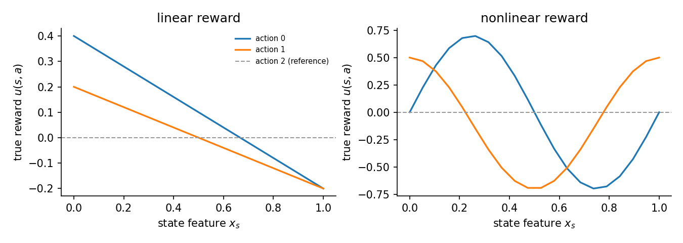
The environment is a 3-action ergodic MDP with 20 states, \(\beta=0.95\), \(\sigma=1\). Each state has a scalar feature \(x_s \in [0,1]\). Action 2 is a zero-reward reference action: its feature is identically zero, \(\phi(s,2) \equiv 0\), so its true reward is 0. This is a location normalization in the Magnac-Thesmar sense; it point-identifies the reward level. All three estimators pin \(u(s,2) = 0\), the two MPEC methods through the feature map and the anchor, and GLADIUS through its anchor argument.

Reward RMSE is reported over the estimated actions \(\{0,1\}\) only. The reference column is a free zero in both truth and estimate, so including it would mechanically lower the error and flatter the numbers; it is excluded. Value RMSE is computed against the soft-Bellman oracle value of the true reward and is comparable across all three methods.

Two reward regimes are studied.

• Linear reward. The true reward is affine in the feature, \(u(s,a) = \phi(s,a)^\top \theta\). The tabular MPEC is fed the same affine feature map, so it is correctly specified.

• Nonlinear reward. The true reward is a wave in the feature, \(u(s,0) = 0.7 \sin 2\pi x\) and \(u(s,1) = 0.6 \cos 2\pi x - 0.1\). The tabular MPEC is fed a reduced \((1, x)\) map per action and is therefore misspecified: an affine function cannot fit a wave.

Results

Each cell is fit on 16,000 observations from a simulated panel. Reward RMSE is over the estimated actions \(\{0,1\}\); value RMSE is against the soft-Bellman oracle. The Bellman residual is reported for neural MPEC, where the equation holds only as a penalty; tabular MPEC enforces it exactly to solver tolerance, and GLADIUS enforces a model-free consistency condition that is not comparable.

Linear reward.

Estimator	Reward RMSE	Value RMSE	Max Bellman residual
neural MPEC	0.165	0.341	0.0076
tabular MPEC	0.021	0.210	exact (hard constraint)
GLADIUS	0.185	2.608	model-free

Nonlinear reward.

Estimator	Reward RMSE	Value RMSE	Max Bellman residual
neural MPEC	0.175	0.390	0.0012
tabular MPEC	0.492	1.822	exact (hard constraint)
GLADIUS	0.480	4.506	model-free

The neural MPEC residual is on the order of \(10^{-3}\) in both cells, so the soft penalty does hold the learned value close to its own Bellman image: the network is near equilibrium, not merely fitting choices.

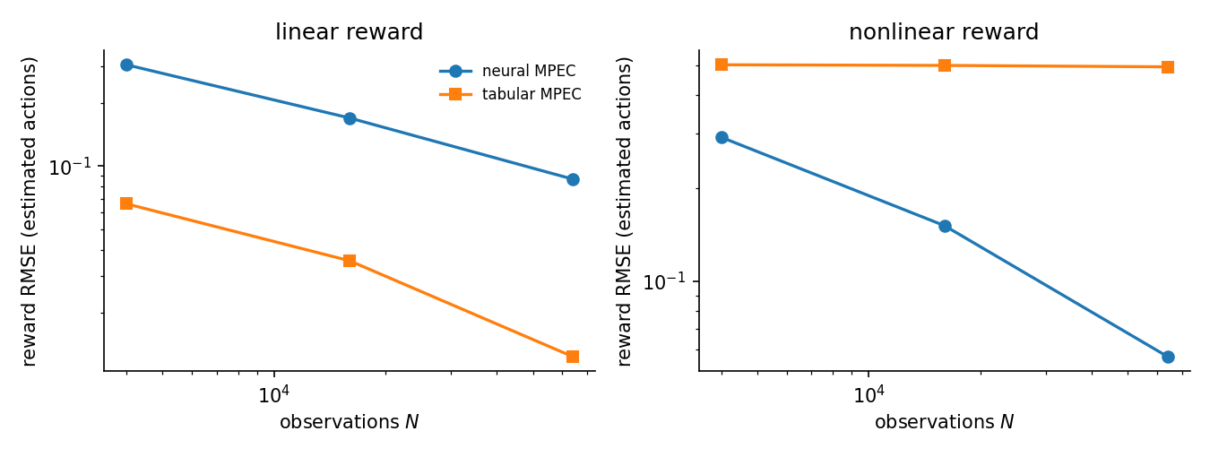
The reward error is best read against sample size. The data-scaling sweep below fits neural and tabular MPEC at \(N = 4{,}000\), \(16{,}000\), and \(64{,}000\) observations and records reward RMSE.

Regime	Method	N = 4k	N = 16k	N = 64k
linear	neural MPEC	0.304	0.170	0.087
linear	tabular MPEC	0.066	0.035	0.012
nonlinear	neural MPEC	0.292	0.151	0.057
nonlinear	tabular MPEC	0.502	0.500	0.494

(The scaling sweep draws a fresh panel, so the linear neural value at 16k, 0.170, is a separate draw from the 0.165 in the table above.)

In the linear regime both curves fall at roughly the root-\(N\) rate, the signature of a consistent estimator. The tabular MPEC sits below the neural one throughout: four pooled parameters are estimated more precisely than a flexible per-state reward, so when the affine specification is correct, the parametric method is more efficient.

In the nonlinear regime the neural curve keeps falling toward zero while the tabular curve is flat at about 0.50. That plateau is a bias floor, not noise: the affine map cannot represent the wave, and more data cannot remove an approximation error. The flexible neural reward recovers the wave and its error keeps shrinking.

Both patterns are textbook behavior for a sample-average estimator. Each MPEC variant is a sample-average approximation of the same population problem. The reward parameters are chosen subject to the Bellman fixed point, and the log-likelihood is estimated from the panel. Shapiro and Xu (2005) show that such constrained estimators are consistent. The sample objective converges to its population counterpart. The root-\(N\) decline in the linear regime is that consistency. The nonlinear plateau is the standard bias floor under misspecification. Consistency cannot cure it, because an affine model cannot represent the wave at any sample size.

It is worth flagging what does not happen here. Koiso and Otani (2024) estimate a sequential-search model by MPEC. At the top of their sweep the pattern reverses. Their estimator had higher bias and error at the larger sample and struggled to find local optima. It got worse with more data. Our linear MPEC improves monotonically across the sweep instead. The difference is the shape of the likelihood. Their search likelihood is a product of smoothed inequality indicators. It is far more non-convex than the smooth soft-Bellman logit likelihood used here. The next section tests that surface directly.

How the three compare

The comparison turns on three axes: the reward form (linear versus neural), whether the transitions are used (known \(P\) versus model-free), and how the Bellman condition is imposed (hard constraint versus soft penalty).

Under a correct linear specification the parametric tabular MPEC is the most efficient method, with the lowest reward RMSE (0.021 versus 0.165) and the lowest value RMSE (0.210 versus 0.341). Pooling the reward into four parameters beats estimating a flexible per-state reward when the four parameters are the right ones. Neural MPEC is still consistent, its reward RMSE falling at root-\(N\), but it pays a variance price for flexibility it does not need here.

Under misspecification the ranking flips. The tabular MPEC reward error plateaus at a bias floor near 0.50 that no amount of data removes, while neural MPEC keeps the reward error falling as it fits the wave. This is the case for which neural flexibility exists: when the analyst does not know the functional form, a method that can represent it avoids a fixed approximation error.

Both known-\(P\) methods recover the value function far better than the model-free GLADIUS, with value RMSE around 0.2 to 0.4 against roughly 2.6 to 4.5. That gap is the cost of not using the known transitions. GLADIUS must learn the expected-continuation operator from data instead of computing it. Its reward is in a different, model-free parameterization because it never uses \(P_a(s,s')\). Its reward RMSE is shown as a model-free reference, not a like-for-like structural comparison with the two known-\(P\) methods.

Local-optima robustness

The cautions about MPEC come from Iskhakov et al. (2016) and the large-sample results in Koiso and Otani (2024). They warn that a constrained estimator can report success at a point that is not the global optimum. Each estimate above comes from a single optimizer start. A different start could in principle land elsewhere.

To separate optimization robustness from sampling noise, one linear-cell panel of 16,000 observations is held fixed and only the start is varied. Linear MPEC is run from \(K=10\) random reward starts, \(\theta_0 \sim \mathcal{N}(0, 0.5^2)\). With each start the value vector is initialized at its own Bellman fixed point, so every run begins feasible. Neural MPEC is run from \(K=10\) random network initializations.

Method	Reward RMSE: mean ± std (min / max)	Optimization diagnostic
linear MPEC	0.0209 ± 0.0005 (0.0204 / 0.0215)	10/10 converged, max constraint violation 9.9e-7, max parameter std across starts 5.7e-4
neural MPEC	0.1648 ± 0.0001 (0.1645 / 0.1650)	max Bellman residual 1.6e-2 across the 10 starts

Both methods are effectively start-independent on this data-generating process. The ten linear-MPEC starts are scattered across reward space. They all converge to the same maximum-likelihood point. The reward RMSE varies by about \(10^{-3}\) and the recovered parameters by under \(10^{-3}\), and every run is feasible to solver tolerance. The neural starts are tighter still. This is the opposite of the Koiso-Otani local-optima struggle. It is the empirical complement to the consistency argument. On the smooth soft-Bellman likelihood the constrained problem has a well-behaved surface, so the single-start estimates do not depend on a lucky initialization. The warning still binds for harder problems. Larger state spaces, discount factors near one, or sharply non-convex likelihoods are exactly where this check earns its place.

Estimators

The three runner functions, lightly trimmed.

def run_neural_mpec(env, obs_states, obs_actions, *, width=32, depth=2, rho=1.0,
                    epochs=4000, lr=5e-3, seed=0) -> dict:
    """Co-train (u_theta, V_phi) with NLL + exact (known-P) Bellman-residual penalty."""
    S, A = env.num_states, env.num_actions
    onehot = jnp.eye(S, dtype=jnp.float64)
    T = jnp.asarray(env.transition_matrices, dtype=jnp.float64)
    obs_s = jnp.asarray(np.asarray(obs_states), dtype=jnp.int32)
    obs_a = jnp.asarray(np.asarray(obs_actions), dtype=jnp.int32)
    w = jnp.ones(S, dtype=jnp.float64) / S  # uniform collocation over the full grid

    key = jax.random.PRNGKey(seed)
    k_r, k_v = jax.random.split(key)
    model = NeuralMPEC(reward=RewardNet(S, A, width, depth, key=k_r),
                       value=ValueNet(S, width, depth, key=k_v))

    def loss_fn(m, rho_):
        u_all = m.reward.all_actions(onehot)
        V_all = m.value.all_states(onehot)
        EV = jnp.einsum("ast,t->as", T, V_all)
        Q = u_all + BETA * EV.T
        logp = jax.nn.log_softmax(Q / SIGMA, axis=1)
        nll = -logp[obs_s, obs_a].mean()
        resid = V_all - SIGMA * jax.scipy.special.logsumexp(Q / SIGMA, axis=1)
        return nll + 0.5 * rho_ * jnp.sum(w * resid**2), None
    # ... adam loop over `epochs`, then return reward/value RMSE and max residual

def run_tabular_mpec(env, panel, est_features, est_names) -> dict:
    from econirl.estimation.mpec import MPECConfig, MPECEstimator

    util = LinearUtility(feature_matrix=jnp.asarray(est_features), parameter_names=est_names)
    est = MPECEstimator(config=MPECConfig(solver="slsqp", outer_max_iter=200,
                                          constraint_tol=1e-6),
                        compute_hessian=False, verbose=False)
    res = est.estimate(panel, util, env.problem_spec, env.transition_matrices)
    est_R = np.einsum("sak,k->sa", np.asarray(est_features), np.asarray(res.parameters))
    true_R = np.asarray(env.true_reward_matrix)
    A = env.num_actions
    return {
        "reward_rmse": rmse(est_R[:, :A - 1], true_R[:, :A - 1]),
        "value_rmse": rmse(res.value_function, oracle_value(env)),
        "converged": bool(res.converged),
    }

def run_gladius(env, panel) -> dict:
    from econirl.estimation.gladius import GLADIUSConfig, GLADIUSEstimator

    S, A = env.num_states, env.num_actions
    util = LinearUtility(feature_matrix=env.feature_matrix,
                         parameter_names=env.parameter_names)
    est = GLADIUSEstimator(config=GLADIUSConfig(
        q_hidden_dim=128, v_hidden_dim=128, q_num_layers=3, v_num_layers=3,
        max_epochs=500, batch_size=512,
        anchor_action=REF_ACTION, anchor_rewards=tuple(0.0 for _ in range(S)),
        anchor_bellman_mode="anchor_moment", compute_se=False, verbose=False,
    ))
    res = est.estimate(panel, util, env.problem_spec, env.transition_matrices)
    reward_table = np.asarray(res.metadata["reward_table"], dtype=np.float64)
    true_R = np.asarray(env.true_reward_matrix)
    return {
        "reward_rmse": rmse(reward_table[:, :A - 1], true_R[:, :A - 1]),
        "value_rmse": rmse(res.value_function, oracle_value(env)),
        "converged": bool(res.converged),
        "note": "model-free; reward in its own parameterization (no known P)",
    }

Reproduce

python scripts/sim_direct_optimization.py                 # main tables + scaling sweep
python scripts/sim_direct_optimization.py --multistart 10 # also runs the K-start probe

Numbers are written to validation/results/sim_direct_optimization.json; the two figures are written under docs/_static/simulation_studies/ (direct_optimization_rewards.png and direct_optimization_scaling.png). The --multistart K flag adds a multistart block to the JSON with the per-start reward RMSE, convergence, and constraint-violation records.