UFXP
Unnested fixed point (UFXP) is a structural estimator for dynamic discrete choice models that recovers primitive reward parameters without solving a dynamic program inside the parameter search. The value-function dependence of Bellman’s first-order conditions is removed by dual fixed points computed once from the empirical choice probabilities. For linear utility with optimal weighting the estimator reduces to a single closed-form solve that attains the same asymptotic efficiency as maximum likelihood.
Read this page as an unnested route to the same finite structural reward target. The method replaces repeated Bellman solves with estimating equations built from empirical choice probabilities.
Source Papers
The estimator follows Bray, which introduces the unnested fixed-point construction and the dual representation of linear functionals of the value function. Oguz and Bray (2026) present the optimally weighted form (OUFXP), prove its asymptotic efficiency equivalence to maximum likelihood, and apply the construction to training neural-network utility functions inside dynamic discrete choice models. The linear-utility case implemented in this package is the default OUFXP path.
Notation
Throughout, \(s\) indexes the discrete state and \(a\) the discrete action, observed for individual \(i\) in period \(t\). The vector \(\phi(s, a)\) collects the known reward features and \(\theta\) the reward parameters to be estimated. The discount factor is \(\beta\), the logit shock scale is \(\sigma\), and \(A\) denotes the reference action used to form log-odds ratios. The transition kernel \(P_a(s, s')\) gives the probability of moving to \(s'\) from \(s\) under action \(a\), stored in \((A, S, S)\) orientation. The empirical conditional choice probability is \(\hat{P}_a(s)\), the CCP-weighted transition is \(F_{\hat{P}} = \sum_a \operatorname{diag}(\hat{P}_a) F_a\), and \(V_{\hat{P}}(s)\) is the value of following the empirical policy. The CCP-weighted feature matrix is \(\Phi_{\hat{P}} = \sum_a \operatorname{diag}(\hat{P}_a) \Phi_a\), where \(\Phi_a\) is the \((S, K)\) slice of \(\phi(s, a)\) at action \(a\). The policy-entropy correction is \(\operatorname{ent}(s) = -\sigma \sum_a \hat{P}_a(s) \log \hat{P}_a(s)\). The dual vector \(\lambda\) satisfies \(\lambda = w + \beta F_{\hat{P}}^\top \lambda\) for a given functional weight \(w\). The integrated value function is \(V_\theta(s)\), the choice-specific value is \(Q_\theta(s, a)\), and the conditional choice probability, the policy, is \(\pi_\theta(a \mid s)\).
Model
The observed data are state, action, and next-state trajectories \((s_{it}, a_{it}, s_{i,t+1})\). The flow payoff is linear in the features:
With discount factor \(\beta\) and logit shock scale \(\sigma\), the integrated value function solves the soft Bellman fixed point:
The choice-specific value is:
The implied conditional choice probability follows the logit rule:
Under any fixed policy \(P\), the value of following that policy has the closed matrix form
Under policy \(P\), the soft-Bellman equation \(V_P(s) = \sum_a P_a(s)[u_\theta(s,a) - \sigma \log P_a(s)] + \beta \sum_{s'} F_P(s,s') V_P(s')\) is a linear system in \(V_P\). In matrix form: \((I - \beta F_P) V_P = \sum_a P_a \circ (u_\theta(\cdot, a) - \sigma \log P_a)\), which inverts to the stated formula. This is the representation used to derive the estimating equations when \(P\) is replaced by the empirical CCPs \(\hat{P}\).
The canonical instance is Rust’s bus-engine replacement model. A bus operator decides each period whether to keep a deteriorating engine or pay a flat cost to replace it. The dynamic program links today’s choices to tomorrow’s states, so observed choices carry information about the structural costs.
Identification
This is the section that says when those empirical choice-probability equations identify the structural reward parameters.
UFXP point-identifies the reward parameters \(\theta\) under the following assumptions.
Conditional independence (CI). The observed state transition is Markov in the current state and action and does not depend on the current logit shock.
Additive separability (AS). The per-period payoff is the systematic reward plus an additive choice-specific shock, drawn independently across choices as Type-I extreme value with fixed scale \(\sigma\).
Exogenous transitions. The transition kernel \(P_a(s, s')\) is supplied or estimated in a first stage, outside the moment system.
Reward normalization. The reward level and scale need an anchor. The reference action \(A\) anchors the log-odds parameterization, and the logit scale \(\sigma\) is held fixed.
Action-dependent feature rank. The reward features must vary across actions. The feature rank must equal the number of parameters. State-only features copied across actions collapse the action contrasts and leave \(\theta\) unidentified.
These hold inside a finite discrete state space, a stationary environment with expected-utility maximization, and a known, fixed discount factor \(\beta\). Given them, \(\theta\) is point-identified. Identification weakens under thin action support, an invalid normalization anchor, or a transition tensor supplied in the wrong orientation.
Estimator
Under logit shocks the log-odds of any two actions at a state equal the difference of their choice-specific values. For any state \(s\) and action \(a \neq A\), the soft Bellman first-order condition is
The obstacle is \(V_{\hat{P}}\), which appears to require a linear solve per candidate \(\theta\). Proposition 2 of Oguz and Bray (2026) removes it: any linear functional \(w^\top V_{\hat{P}}\) has the dual representation
where \(\lambda\) depends only on \(\hat{P}\), \(\beta\), and the transitions, not on \(\theta\). The identity follows from the policy-value equation \((I - \beta F_{\hat{P}}) V_{\hat{P}} = u_{\hat{P}}\): left-multiplying by \(\lambda^\top\) and using the dual fixed point \(\lambda = w + \beta F_{\hat{P}}^\top \lambda\) gives \(w^\top V_{\hat{P}} = \lambda^\top u_{\hat{P}}\) directly. One matrix factorization of \((I - \beta F_{\hat{P}}^\top)\), computed once before the parameter search, removes the value function entirely. Substituting this dual representation, the first-order condition at state \(s\) and action \(a \neq A\) becomes affine in \(\theta\):
where
with \(\rho(s) = \sigma\log(\hat{P}_a(s)/\hat{P}_A(s))\) the log-odds vector (stacked over \(a \neq A\)), \(\Delta F(s) = (F_a - F_A)\) the differenced transitions, \(v_{\text{ent}} = (I - \beta F_{\hat{P}})^{-1}\,\text{ent}\) the entropy-correction value, and \(dV = (I - \beta F_{\hat{P}})^{-1}\Phi_{\hat{P}}\) the value gradient with respect to \(\theta\).
The value gradient \(dV\) comes from differentiating the policy-value identity. The linear policy-value identity is \(V_{\hat{P}} = (I - \beta F_{\hat{P}})^{-1}[\sum_a \hat{P}_a \circ (\phi(\cdot,a)^\top\theta - \sigma \log \hat{P}_a)]\). Differentiating with respect to \(\theta\) at fixed \(\hat{P}\) gives
because the only \(\theta\)-dependent term inside the brackets is \(\sum_a \hat{P}_a \circ \phi(\cdot,a)^\top\theta = \Phi_{\hat{P}}\,\theta\), so its \(\theta\)-derivative is \(\Phi_{\hat{P}}\) exactly. This is the shared implicit-differentiation step: the matrix \((I - \beta F_{\hat{P}})\) is \(\theta\)-free, so no chain rule through the inverse is needed. The result makes \(dV\) constant in \(\theta\), which is what enables the closed-form solve.
Separating the \(\theta\)-dependent part of \(V_{\hat{P}}\) using \(\partial V_{\hat{P}}/\partial\theta = dV\) and the constant entropy-correction value \(v_{\text{ent}} = (I - \beta F_{\hat{P}})^{-1}\,\text{ent}\), write \(V_{\hat{P}} = dV\,\theta + v_{\text{ent}}\). Substituting into the first-order condition gives \(\sigma \log(\hat{P}_a/\hat{P}_A) = \Delta\phi(s)^\top\theta + \beta\,\Delta F(s)(dV\,\theta + v_{\text{ent}})\), which rearranges to \(y(s) = G(s)\,\theta + \varepsilon(s)\) with \(G\) and \(y\) as defined above.
Both \(v_{\text{ent}}\) and \(dV\) are independent of \(\theta\) and are precomputed from a single factorization of \((I - \beta F_{\hat{P}})\).
The optimally weighted estimator assigns each supported state a weight matrix:
where \(\Sigma(s) = \operatorname{diag}(\hat{P}(s)) - \hat{P}(s)\hat{P}(s)^\top\) is the multinomial covariance of the empirical CCPs, \(\Gamma(s)\) is the Jacobian of the inverse-CCP map with \(\Gamma_{a,b}(s) = \sigma\,\delta_{a,b}/\hat{P}_a(s) - \sigma\,\delta_{b,A}/\hat{P}_A(s)\) (where \(\delta\) is the Kronecker delta, \(a\) indexes the \(A-1\) non-reference actions, and \(b\) indexes all \(A\) actions), and \(\eta(s) = N(s)/N\) is the state’s sample share. Setting the weighted moments to zero gives \(\sum_s z(s)^\top G(s)\,\theta = \sum_s z(s)^\top y(s)\), so the closed-form solution is:
By Theorem 2 of Oguz and Bray (2026), this estimator is as asymptotically efficient as maximum likelihood. Standard errors come from the efficient moment variance:
At optimal weights, the efficient-GMM sandwich \(V = J^{-1}\Omega J^{-\top}\) collapses to \(D^{-1}/N\) because the moment variance \(\Omega = D/N\) at the optimum (Theorem 2 of Oguz and Bray 2026).
Thin states are downweighted by \(\eta(s)\); unvisited states drop out of the moment system entirely.
Algorithm
Algorithm  UFXP (unnested fixed-point estimation, OUFXP default)
Input   panel {(s_it, a_it, s_{i,t+1})}, features phi, transitions P,
        discount beta, logit scale sigma, reference action A
Output  theta_hat, standard errors, policy pi, value V

1   estimate empirical CCPs P-hat state by state (frequency + additive smoothing)
2   factorize (I - beta * F_P-hat)                     # one dense solve; independent of theta
3   dV    := (I - beta * F_P-hat)^{-1} phi_P           # value gradient w.r.t. theta, (S, K)
4   v_ent := (I - beta * F_P-hat)^{-1} ent             # entropy-correction value, (S,)
5   D := 0,  rhs := 0
6   for each supported state s:
7       G(s)     := dphi(s) + beta * dF(s) dV          # moment Jacobian, (A-1, K)
8       y(s)     := logratio(s) - beta * dF(s) v_ent   # moment intercept, (A-1,)
9       Gamma(s) := Jacobian of inverse-CCP map at P-hat(s)         # (A-1, A)
10      Sigma(s) := diag(P-hat(s)) - P-hat(s) P-hat(s)^T           # CCP covariance, (A, A)
11      z(s)     := [Gamma(s) Sigma(s) Gamma(s)^T / eta(s)]^{-1} G(s)  # optimal weight
12      D   += G(s)^T z(s)
13      rhs += z(s)^T y(s)
14  theta_hat := D^{-1} rhs                            # closed-form weighted moment solve
15  solve  V_theta_hat = T_theta_hat V_theta_hat       # one value iteration at theta_hat
16  return theta_hat, D^{-1}/N as standard errors, pi_theta_hat, V_theta_hat
The default variant is weights="optimal" (the OUFXP form of Oguz and Bray 2026):
the single factorization in step 2 removes the value function from the estimation
problem, and the per-state optimal weights in steps 6-13 deliver maximum-likelihood
efficiency. An alternative variant is weights="random" (plain UFXP): \(m\) random
projection matrices \(Z_i\) replace the optimal weights; \(m\) dual vectors \(\lambda_i\)
are pre-computed from the same single factorization via Proposition 2, and the
estimator solves an ordinary least-squares problem. Plain UFXP is consistent but
less efficient and produces no standard errors; it is retained for comparison with
the paper’s baseline construction.
Applicability
Applicable when |
Prefer an alternative when |
|---|---|
States and actions are discrete. |
The state space makes the dense \((I - \beta F_{\hat{P}})\) factorization binding. |
Transitions are known or can be estimated first. |
Transition estimation is the main modeling challenge. |
The reward has a compact parametric form. |
The reward must be high-dimensional or neural. |
Maximum-likelihood-grade efficiency is required at low cost. |
An exact finite-sample MLE benchmark is required (use NFXP). |
Most states are visited in the data. |
State coverage is very thin everywhere (prefer NFXP, which pools all observations through the likelihood). |
Counterfactual policy analysis is central. |
Only fitted choice probabilities are required. |
UFXP sits with NFXP, CCP, and MPEC in the structural family. Against NFXP the trade is direct: NFXP is the exact finite-sample maximum likelihood estimator; UFXP is its asymptotic equal at almost no cost, because no dynamic program is solved inside the search. Against CCP, UFXP shares the sensitivity to thin state coverage (both invert empirical CCPs state by state), but UFXP weights all of Bellman’s restrictions optimally rather than inverting once, and its optimal weighting restores maximum-likelihood efficiency. NNES and TD-CCP become attractive when approximate methods are acceptable; UFXP is the preferred structural alternative when the state space makes NFXP’s repeated solves expensive.
Usage
from econirl.datasets import load_rust_bus, rust_bus_reward_spec
from econirl import UFXP

df = load_rust_bus()

model = UFXP(n_states=90, discount=0.9999, utility=rust_bus_reward_spec(90))
model.fit(df, state="mileage_bin", action="replaced", id="bus_id")

print(model.params_)
print(model.summary())
Counterfactual analysis re-solves the fitted dynamic program under a changed primitive:
cf = model.counterfactual(replacement_cost=4.0)   # raise the replacement cost
print(cf.params)
print(cf.policy)                       # new replacement probability by state
The fitted policy gives the replacement probability by state:
print(model.predict_proba([0, 10, 50, 89]))
The Quick Start page documents the full set of fitted
attributes, weighting modes, and the full UFXPEstimator API.
Evidence
Parameter recovery is measured on a synthetic benchmark with known rewards, transitions, policies, values, Q functions, and Type A, Type B, and Type C counterfactual oracles. The figure below is a Monte-Carlo study over 100 replications: the panel is resimulated and refit on a fresh seed each time, and each parameter is plotted as its recovered mean and 95% interval against the true value.
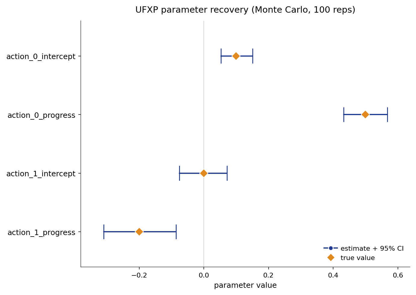
Recovery statistics are over a Monte-Carlo run of 100 replications.
Parameter |
True |
Recovered (mean) |
95% interval |
|---|---|---|---|
|
0.10 |
0.103 |
[0.053, 0.151] |
|
0.50 |
0.494 |
[0.432, 0.567] |
|
0.00 |
0.003 |
[-0.076, 0.071] |
|
-0.20 |
-0.198 |
[-0.310, -0.086] |
Across the 100 replications the true value sits inside the 95% interval for every parameter, and the mean estimate is close to the truth.
Behavioral fit and counterfactual regret on the same cell, against the known oracle objects:
Metric |
Value |
|---|---|
Policy total variation |
0.0050 |
Value RMSE |
0.0170 |
Type A regret (reward shift) |
0.000161 |
Type B regret (transition change) |
0.000300 |
Type C regret (action removed) |
0.000078 |
The regrets are small because the recovered reward is close enough to the truth that re-solving the intervened model reproduces almost the same policy as the oracle. For the full cross-estimator comparison, see the bus engine simulation study.
References
Source papers:
Bray, R. L. “Unnesting the Fixed Point in the Estimation of Dynamic Programs.” Working paper, SSRN 3307175. reference entry.
Oguz, E., and Bray, R. L. (2026). “Training Neural Networks Embedded in Dynamic Discrete Choice Models.” Working paper, arXiv 2604.09736. reference entry.
Implementation and reproduction:
Estimator source:
econirl.estimation.ufxp.sklearn wrapper:
econirl.UFXP.Validation runner:
validation/estimators/ufxp/run.py.Results file:
ufxp.json.
Pages: